Missing Data: 2 Big Problems With Mean Imputation

While it may be simple at first sight, the truth is that mean imputation can be dangerous. 

The truth is that mean imputation is a very popular solution to deal with missing data. While it comes with many obstacles, the main reason why we stick to his solution is that it is easy. However, you need to keep in mind that there are many other alternatives to mean imputation that can deliver more accurate estimates and standard errors. 

Check out all the stats calculators you need.

What Is Mean Imputation?

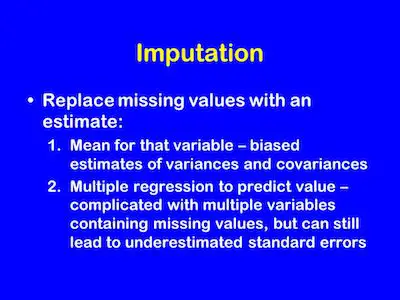
Simply put, man imputation is just the replacement of a missing observation with the mean of the non-missing observations for that specific variable. 

The Problems With Mean Imputation

#1: Mean Imputation Doesn’t Preserve The Relationships Among Variables:

If you think about it, imputing the mean preserves the mean of the observed data. So, when you have data that is missing completely at random, the estimate of the mean remains unbiased. And this is a good thing. 

In addition, when you input the mean, you can keep your sample size up to the full sample size. And this is also a good thing. 

How to deal with missing data in statistics?

So, we can then state that if you are only estimating means (which rarely happens), and if the data are missing completely at random, mean imputation will not bias your parameter estimate.

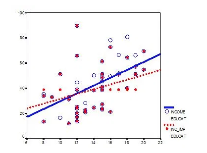
Since most research studies are interested in the relationship among variables, mean imputation is not a good solution. The following graph illustrates this well:

This graph shows hypothetical data between X=years of education and Y=annual income in thousands with n=50.

The blue circles are the original data, and the solid blue line indicates the best fit regression line for the full data set. 

The correlation between X and Y is r = .53.

We randomly deleted 12 observations of income (Y) and substituted the mean. The red dots are the mean-imputed data.

Learning the generative and analytical models for data analysis.

Blue circles with red dots inside them represent non-missing data. Empty Blue circles represent the missing data. 

So, if you look across the graph at Y = 39, you will see a row of red dots without blue circles. These represent imputed values.

The dotted red line is the new best fit regression line with the imputed data. As you can see, it is less steep than the original line. Adding in those red dots pulled it down.

The new correlation is r = 0.39. That’s a lot smaller than 0.53.

The real relationship is quite underestimated.

Of course, in a real data set, you wouldn’t notice so easily the bias you’re introducing. This is one of those situations when you are trying to solve the lowered sample size, but you create a bigger problem.

Looking at OLS (Ordinary Least Squares) assumptions.

#2: Mean Imputation Leads To An Underestimate Of Standard Errors:

You need to know that any statistic that uses the imputed data will have a standard error that’s too low. So, you may get the same mean from mean-imputed data that you would have gotten without the imputations. And yes, there are circumstances where that mean is unbiased. Even so, the standard error of that mean will be too small.

Because the imputations are themselves estimates, there is some error associated with them. But your statistical software doesn’t know that. It treats it as real data.

Ultimately, because your standard errors are too low, so are your p-values. Now you’re making Type I errors without realizing it.

That’s not good.