Home

Category : Blog

Preparing Data For Analysis Is Crucial

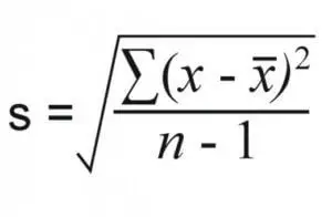
One of the most important aspects of statistics is the data that you have. The reality is that when you get a bunch of data, you need to take the time o prepare it. While this may seem a very simple and fast task, the truth is that it isn’t. Preparing data can be incredibly slow but is extremely important before you start with its analysis.

Looking to run statistic models?

Something that most people tend to assume is that preparing data can b very fast. So, if you are working with a client, it’s important that you explain to him that this is a slow process. Nevertheless, even if you say it will take you one hour, your client will still have unrealistic expectations that it will be a lot faster.

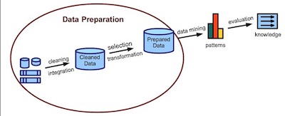
The time-consuming part is preparing the data. Weeks or months is a realistic time frame. Hours is not. Why? There are three parts to preparing data: cleaning it, creating necessary variables, and formatting all variables.

Preparing Data For Analysis Is Crucial

#1: Data Cleaning:

Data cleaning means finding and eliminating errors in the data. How you approach it depends on how large the data set is, but the kinds of things you’re looking for are:

Impossible or otherwise incorrect values for specific variables
Cases in the data who met exclusion criteria and shouldn’t be in the study
Duplicate cases
Missing data and outliers
Skip-pattern or logic breakdowns
Making sure that the same value of string variables is always written the same way (male ≠ Male in most statistical software).

You can’t avoid data cleaning and it always takes a while, but there are ways to make it more efficient. For example, one way to find impossible values for a variable is to print out data for cases outside a normal range.

This is where learning how to code in your statistical software of choice really helps. You’ll need to subset your data using IF statements to find those impossible values. But if your data set is anything but small, you can also save yourself a lot of time, code, and errors by incorporating efficiencies like loops and macros so that you can perform some of these checks on many variables at once.

Understanding the basics of principal component analysis.

#2: Creating New Variables:

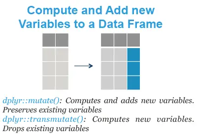
Once the data are free of errors, you need to set up the variables that will directly answer your research questions.

It’s a rare data set in which every variable you need is measured directly.

So you may need to do a lot of recoding and computing of variables.

Examples include:

Creating change scores
Creating indices from scales
Combining too-small-to-use categories of nominal variables
Centering variables
Restructuring data from wide format to long (or the reverse)

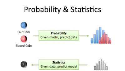
An introduction to probability and statistics.

#3: Formatting Variables:

Both original and newly created variables need to be formatted correctly for two reasons:

So your software works with them correctly. Failing to format a missing value code or a dummy variable correctly will have major consequences for your data analysis.
It’s much faster to run the analyses and interpret results if you don’t have to keep looking up which variable Q156 is.

Learn the basics of probability.

Examples include:

Setting all missing data codes so missing data are treated as such
Formatting date variables as dates, numerical variables as numbers, etc.
Labeling all variables and categorical values so you don’t have to keep looking them up.

1-07-2021 | Comments Off

The Difference Between Model Assumptions, Inference Assumptions, And Data Issues

One of the things that you may have never noticed before is that the list of assumptions for linear regression that you find on textbooks, lecture notes, or websites may be different. But why does this happen?

Discover the best statistics calculators online.

The reality is that authors use different terminology. So, while they are using the same assumptions, they look different. However, it’s important to keep in mind that sometimes they’re including not only model assumptions but inference assumptions and data issues. While they are all important, it’s even more important to understand the role of each can help you understand what applies in your situation.

Model Assumptions

Simply put, the model assumptions are all about the specification and performance of the model for estimating the parameters well.

1. The errors are independent of each other

2. The errors are normally distributed

3. The errors have a mean of 0 at all values of X

4. The errors have constant variance

5. All X are fixed and are measured without error

6. The model is linear in the parameters

7. The predictors and response are specified correctly

8. There is a single source of unmeasured random variance

Learn more about the t-test and the f-test.

Notice that not all these model assumptions will be stated explicitly not to mention that you can’t check them all. Ultimately, you need to make sure that you included all the “correct” predictors. Nevertheless, you shouldn’t skip the step of checking what you can. And for those you can’t, take the time to think about how likely they are in your study and report that you’re making those assumptions.

Assumptions About Inference

Sometimes the assumption is not really about the model, but about the types of conclusions or interpretations that you can make about the results.

These assumptions allow the model to be useful in answering specific research questions based on the research design. They’re not about how well the model estimates parameters.

Check out the analysis of variance explained.

As you know, studies are designed to answer specific research questions. And they can only do that if these inferential assumptions hold. But if they don’t, it doesn’t mean the model estimates are wrong, biased, or inefficient. It simply means you have to be careful about the conclusions you draw from your results. Sometimes this is a huge problem.

But these assumptions don’t apply if they’re for designs you’re not using or inferences you’re not trying to make. This is a situation when reading a statistics book that is written for a different field of application can really be confusing. They focus on the types of designs and inferences that are common in that field.

It’s hard to list out these assumptions because they depend on the types of designs that are possible given ethics and logistics and the types of research questions. But here are a few examples:

1. ANCOVA assumes the covariate and the IV are uncorrelated and do not interact.

2. The predictors in a regression model are endogenous.

3. The sample is representative of the population of interest.

Data Issues That Are Often Mistaken For Assumptions

One of the things that tend to occur to many people is that their list of assumptions includes data issues that are a little different. However, they are still important. After all, they affect how you interpret the results as well as they impact how well the model performs.

What is a partial correlation?

When a model assumption fails, you can sometimes solve it by using a different type of model. Data issues generally stay around. That’s a big difference in practice.

Here are a few examples of common data issues:

1. Small Samples

2. Outliers

3. Multicollinearity

4. Missing Data

5. Truncation and Censoring

6. Excess Zeros

1-06-2021 | Comments Off

T-Test And F-Test: Fundamentals Of Test Statistics

As you already know, statistics is all about coming up with models to explain what is going on in the world.

But how good are we at that? After all, numbers are only good for so many things, right? How do we know if they are telling the right story? This is why you need to use test statistics.

The main goal of a test statistic is to determine how well the model fits the data. Think of it a little like clothing. When you are in the store, the mannequin tells you how the clothes are supposed to look (the theoretical model). When you get home, you test them out and see how they actually look (the data-based model). The test-statistic tells you if the difference between them is significant.

Discover the best statistics calculators.

Simply put, test statistics calculate whether there is a significant difference between groups. Most often, test statistics are used to see if the model that you come up with is different from the ideal model of the population. For example, do the clothes look significantly different on the mannequin than they do on you?

Let’s take a look at the two most common types of test statistics: t-test and F-test.

T-Test And Comparing Means

The t-test is a test statistic that compares the means of two different groups. There are a bunch of cases in which you may want to compare group performance such as test scores, clinical trials, or even how happy different types of people are in different places. As you can easily understand, different types of groups and setups call for different types of tests. The type of t-test that you may need depends on the type of sample that you have.

Understanding the basics of probability.

If your two groups are the same size and you are taking a sort of before-and-after experiment, then you will conduct what is called a dependent or Paired Sample t-test. If the two groups are different sizes or you are comparing two separate event means, then you conduct an Independent Sample t-test.

Overall speaking, a t-test is a form of statistical analysis that compares the measured mean to the population mean, or a baseline mean, in terms of standard deviation. Since we are dealing with the same group of people in a before-and-after kind of situation, you want to conduct a dependent t-test. You can think of the without scenario as a baseline to the with scenario.

F-Test Statistic

Sometimes, you want to compare a model that you have calculated to a mean. For example, let’s say that you have calculated a linear regression model. Remember that the mean is also a model that can be used to explain the data.

Learn the measures of position.

The F-Test is a way that you compare the model that you have calculated to the overall mean of the data. Similar to the t-test, if it is higher than a critical value then the model is better at explaining the data than the mean is.

Before we get into the nitty-gritty of the F-test, we need to talk about the sum of squares. Let’s take a look at an example of some data that already has a line of best fit on it.

The F-test compares what is called the mean sum of squares for the residuals of the model and the overall mean of the data. Party fact, the residuals are the difference between the actual, or observed, data point and the predicted data point.

Understanding the measures of dispersion.

In the case of graph (a), you are looking at the residuals of the data points and the overall sample mean. In the case of graph (c), you are looking at the residuals of the data points and the model that you calculated from the data. But in graph (b), you are looking at the residuals of the model and the overall sample mean.

The sum of squares is a measure of how the residuals compare to the model or the mean, depending on which one we are working with.

12-24-2020 | Comments Off

Analysis Of Variance Explained

Analysis of variance which is more commonly called ANOVA, is just a statistical method that is designed to compare means of different samples.

Simply put, it’s a very easy way to compare how different samples in an experiment differ from one another if they differ at all. It is similar to a t-test except that ANOVA is generally used to compare more than two samples.

Discover everything you need to know about statistics.

As you probably already know, each time you do a t-test, you actually compound the error. This means that the error gets larger for every test you do. So, what starts as a 5% error for one test can turn into a 14% error for 3 tests!

ANOVA is a method that takes these little details into account by comparing the samples not only to each other but also to an overall Grand Mean, Sum of Squares (SS), and Mean Square (s2). It also compares error rates within the groups and between the groups. ANOVA tests the hypothesis that the means of different samples are either different from each other or the population.

The Details

When you use ANOVA, you are testing whether a null hypothesis is true, just like regular hypothesis testing. The difference is that the null hypothesis states that the means of each group are equal. You would state it something like X1 = X2 = X3. ANOVA would tell you that one or all of them are not equal.

What is partial correlation?

You also need to keep in mind that ANOVA relies on the F-distribution. Simply put, the F-distribution compares how much variance there is in the groups to how much variance there is between the groups.

If the null hypothesis is true, then the variances would be about equal, though we use an F-table of critical values in a similar way to a t-test to determine if the values are similar enough.

Analysis of variance compares means, but to compare them all to each other we need to calculate a Grand Mean.

The Grand Mean, GM, is the mean of all the scores. It doesn’t matter what group they belong to, we need a total mean for comparison.

Understanding the basics of principal component analysis.

The Sum of Squares, SS, is what you get when you add up all the squared standard deviations. We use this value to calculate the Mean Square of Treatment, MStreat, which is the sum of squares divided by the degrees of freedom in the sample (N – number of groups). It tells you the amount of variability between the groups.

The final detail that we are going to talk about is the Error Sum of Squares, SSerror, which refers to the overall variance of the samples.

Remember that variance tells you how precise your data is. SSerror is used to calculate the Mean Error Sum of Squares, MSerror. This basically tells us the variability of the data in the group.

An introduction to probability and statistics.

Bottom Line

As you can see, the analysis of variance doesn’t ned to be hard. It just takes a bit more time and a bit more effort from your part.

12-23-2020 | Comments Off

What Is A Partial Correlation?

Correlation isn’t something new to you that are studying statistics. But what about partial correlation?

Let’s take a look at an example so you can fully understand this concept. Imagine that you are trying to lose some weight. So, you will try to change your diet and do exercise at the same time. To ensure that you are covering all aspects, you use an app to keep track of how much you eat and how much exercise you do besides your weight. However, while dieting may be something most people are willing to do, we can’t say the same about exercise. Between the lack of time, not finding a sport you like, lack of motivation, or anything else, you just don’t like to exercise. So, the question that you ask yourself is: if you just change your diet, do you need to exercise as well? Well, to answer this question, you need to use partial correlation, a statistical method.

Looking for the best statistic calculators online?

Partial Correlation

Simply put, a partial correlation is just the correlation between 2 variables when a third variable is held constant.

As we mentioned above, you know that there is a correlation between diet and exercise which is a positive correlation. After all, this means that the better you diet, the more weight you will lose. So, what about the relationship between exercise and weight loss?

As you can easily understand, the relationship between these two variables is negative. While it sounds bad, it really isn’t since the more exercise you do, the more weight you will lose.

Discover the difference between association and correlation.

But what you are trying to get is a complete picture of how both diet and exercise correlate to weight loss. So, in this case, you need to consider the effect exercise has on dieting and weight loss. This is where the partial correlation is useful.

This image shows the relationship between diet and weight loss. The shaded region would be the correlation between these two variables.

This image shows the relationship between exercise and weight loss. The orange region represents the correlation between the two variables.

relationship-between-diet-exercise-and-weight-loss

This is the image that represents what you are after. As you can see, the grey region represents the overall correlation between the three variables. The orange and green shaded regions are still there. These indicate the partial correlations that still explain some of the weight loss; however, the grey region is how they both explain what is going on with weight loss.

These are the different types of correlation.

What Do Partial Correlations Do?

As you probably already know, multiple regression is one way to explain patterns in data using multiple variables. However, these aren’t the same as partial correlations. Remember that multiple regression is a way of explaining how individual variables explain relationships. Partial correlations explain how variables work together to explain patterns in the data.

Discover the difference between correlation and linear regression.

The main benefit of using partial correlations is that they allow you to explain patterns in data. For example, in education, there are different types of engagement (cognitive, behavioral, and emotional if you’re interested) that overlap to affect learning. In movies, the amount of romance, action, and comedy in a movie work together to affect box office sales. All of these could be analyzed with partial correlations.

Ultimately, partial correlations are a way to explain patterns in the data using multiple variables. In this case, you look for how multiple variables overlap to explain patterns in the data and come up with a more accurate and reliable model.

12-15-2020 | Comments Off

Understanding The Basics Of Principal Component Analysis

In case you are studying statistics, at some point, you will cross with the principal component analysis concept.

Discover the best stat calculators online.

Simply put, principal component analysis is just a statistical technique that allows you to do the same thing with data. So, you will be able to try to find which items fo together because they are the result of something you can’t observe directly. For example, imagine that you’re taking a walk in a forest and you see a pile of laves there. The principal component analysis allows you to figure out which leaves come from which tree. So, to do this, you will need to look at the leaves and see which ones are similar and then look for the tree that went with them.

Factors

Factors are just the underlying perceptions or concepts that you can’t directly observe. However, you can observe their effects on different surveys and tests.

Here’s a simple example. You have no idea about how other teachers engage their students in a class since you can’t observe them directly. However, you can design a survey for teachers made of items that represent what research says engagement should like in a class.

Check out our student t value calculator.

Imagine that you made a survey with 20 questions and that the factor you want to measure is student engagement. The survey items represent the effect of engagement. In a scientific sense, you can think of the factor as an independent variable and the items as a dependent variable.

Factor Analysis

As you can easily understand factor analysis is a technique that looks for correlation between items. In case you had a survey of 6 items, the correlations might look like this:

Notice that items x1 – x3 have high correlations with each other while x4 – x6 have high correlations with each other but not x1 – x3. Logically, items x1 – x3 are related and x4 – x6 are related. This means that there are two separate concepts that the items are measuring. Those concepts are the factors.

Looking for an effect size (Cohen’s d) for a student t-test calculator?

However, a simple factor analysis does not take some things into account such as the covariance of the items.

Principal Component Analysis

Simply put, principal component analysis is a more robust and mature version of factor analysis. As you can easily assume, this type of analysis doesn’t only look for correlations of the items but it also looks at correlations between the variance of the items.

Discover our z-score calculator.

The reality is that the variance between the items helps explain how the items are related. For example, if x1 and x4 have a low covariance, then changes in x1 do not explain the changes in x4 very well.

As you can easily understand, principal component analysis has an advantage over traditional factor analysis because it takes into account that the variable may explain each other and how well they do that. If the variances are related, then it makes sense that the items are related.

12-14-2020 | Comments Off

Introduction To Probability And Statistics

There’s no question that probability and statistics are related. Ultimately they can both deliver the answers to questions such as:

How likely are you to flip a coin and it lands on its edge?
How likely is that you wear a blue shirt today?

Among others.

Discover the best stats calculators.

Probability

Simply put, the probability is the likelihood of something happening. This “something” is called an event.

For example, let’s say that you’re playing Dungeons & Dragons. When you roll a D20, getting a 20 is a very good thing most of the time. However, everyone says that this is extremely rare. Yet, in reality, it is just as likely to roll a 20 as a 1. Let’s figure out why.

Complete overview of the most common probability math problems.

When you are trying to figure out probability (P), you are trying to figure out the chance of an event occurring. The probability of an event occurring is usually written as P(event).

In the case of our D&D dice when you roll it you have these outcomes

S = {1, 2, 3, 4, 5, 6, 7, 8, 9, 10, 11, 12, 13, 14, 15, 16, 17, 18, 19, 20}

This means that the likelihood of rolling a number 1 – 20 is 100% while the likelihood of rolling a 21 is 0%. But the events in between are a little different.

Probability is calculated as the total number of desired outcomes ÷ total number of possible outcomes.

Getting Back At Our Example

As we already mentioned above, there are 20 total possible events that can occur on a single roll of a fair D20.

At this time, we are only interested in one of them, 20. Since it is one of 20 possible outcomes:

P(20) = 1/20 = 0.05.

We also already mentioned that it has the same likelihood of a 1 being rolled:

P(1) = 1/20 = 0.05.

Now, rolling a number less than twenty is different. This would be:

P(1, 2, 3, 4, 5, 6, 7, 8, 9, 10, 11, 12, 13, 14, 15, 16, 17, 18, 19) = 19/20 = 0.95

As you can see, it is much more likely.

Summing up, rolling a D20 and getting a 20 is just as likely as rolling a 1. However, the reason 20s are so rare is that you are much more likely to roll a number less than 20.

What is the probability theory?

Statistics

As you already know, statistics is the application of the laws of probability to real, actual data.

If you take the D20 example, this would be when you roll the dice 20 times and collect some data.

When you apply probability to real data, you are trying to determine if the outcome is significantly different from a model that you are generating.

For example, the P(20) = 0.05, so let’s explore that.

Check out our binomial probability calculator.

When you collect data, there are several ways to describe the data that you take. The most common are mean, median, and mode. In the case of statistics, we want to see if our actual data conforms to the model. There are two ways to do this:

#1: Classical Inference:

Classical inference deals with data that have a fixed probability based on the number of cases and events.

#2: Bayesian inference:

Bayesian inference deals with data whose probability is not fixed. That is, the probability is subject to change based on other factors.

12-09-2020 | Comments Off

The Basics Of Probability

Generally speaking, when we talk about probability, we are referring to the likelihood that a certain event will occur.

Discover the best statistics calculators in 2020.

One of the things you need to know about probabilities is that they vary between 0 and 1 (or 0% and 100%). The closer the probability is to zero, the lesser the likelihood the event has of occurring. On the other hand, the closer a probability is to 1, the greater the likelihood the event will occur.

The truth is that since you have some background in statistics, probabilities are not new to you. But even if you’re just starting in statistics, if you look at the weather report for the day and see that there’s a “90% chance of rain,” you know that you should probably bring an umbrella. However, a “10% chance of rain” might prompt you to leave the umbrella at home.

So, where do these numbers come from?

Check out our binomial probability calculator.

Basics Of Probability: Certain Events And Impossible Events

As you can easily understand, when an event has a probability of 1 or 100%, we can call it a certain event. For example, in a coin toss, the probability that the coin lands either heads or tails is 100%. These are the only possible outcomes, and it’s certain that one of them will occur.

On the other hand, an impossible event has a probability of 0 or 0%. An example would the probability of drawing five kings from a fair, standard deck of 52 cards. The reason this event is impossible is because there are only four kings in the deck.

Learn more about the probability theory.

Calculating Theoretical Probability

Imagine now that you have a bag and 8 colored marbles inside, all equal in size, and weight.

If you pick a random bag from the bag, what is the probability that it is the black marble? To determine this, you would need to use the following formula:

Notice that the desired outcome is what you want. In this example, it would b the black marble which means that you only have one desired outcome out of a total of 8 total possible outcomes (8 total marbles).

Therefore the probability that you pick the black marble is ⅛, or 0.125, or 12.5%. We often write this as follows:

P(black) = ⅛

Check out this overview of the most common probability math problems.

Probability And Sample Spaces

Let’s keep using the same example of the bag with 8 marbles inside. The bag and the marbles it contains can be considered a sample space.

Technically speaking, a sample space contains all the values that a random variable can take. This means that it contains all the possible outcomes. So, getting back at our example, all of the outcomes are equally likely.

Basics Of Probability: “Or”

When you are learning probabilities, it is fairly common that you need to work with the word “or”. For example, imagine that you want to find out the probability that you draw a black or a red marble from the bag.

As you can easily understand, this increases your number of desired outcomes since you now may draw a black or a red marble.

Since there is one black marble and two red marbles, the total number of desired outcomes is now three. Since the total number of possible outcomes is unchanged (the number of total marbles is constant), so:

P(black or red) = ⅜

12-08-2020 | Comments Off

Measures Of Position Explained

In statistics, you have to find a way to figure out where a data point or set falls in. So, you need to use measures of position.

Make sure to check out the best online stats calculators.

The reality is that as soon as you know where a data set or model is, you can figure out what to do with it. So, how can you find out where data is and what it means?

Measures Of Position Explained

#1: Percentiles:

There’s no question that percentiles are common measures of position.

To get a percentile, the data is divided into 100 regions. A specific data point will fall in one of those regions and then you assign a percentile to indicate how much data is below that specific data point.

Here’s an example. Let’s say that you took your child to the doctor and they measured her height. Once they had her height, they compared it to the national average. In the case of your child, she is in about the 50% of the national data. This means that she is taller than 50% of girls her age. This means that she is above average.

This is the best online z-score calculator.

As you can see, percentiles are a good way to express the measure of position for large datasets. Many national assessments, such as height and ACT scores, use percentiles as a way to convey where specific scores fall because they are easily interpreted.

#2: Quartiles:

Simply put, quartiles divide the data into four regions. The first region comprises the lowest point in the data to the median of the lower half of the data. The second quartile region is from the median of the lower half of the data to the median of the entire data set. The third region makes up the data from the median of the entire data set to the median of the upper half of the data. The final region is made up of the data from the median of the upper half to the greatest data point.

The key region is known as the interquartile range and it represents the middle 50% of the data. Knowing which quartile a datum falls in gives you a sense of how different the data is. Besides, it is also a get way to identify outliers, the points that are excessively high or low.

Check out the 5 steps for calculating sample size.

#3: Z-Scores:

If there is something you need to know about a-scores is that they’re the most amazing way to identify how a data point differs from the mean.

Simply put, a z-score is a measure of how much the datum or model differs from a standardized mean. Once you calculate a z-score, you can then determine whether it is different enough to be significant. A z-score is calculated as follows:

Since is in terms of standard deviations, it is possible to determine the significant difference.

A quick understanding about factor analysis and how big your sample needs to be.

For example, a datum of a model with a z-score of ± 1.2 means that the datum differs from the mean by 1.2 standard deviations. If the z-score is ± 2.6, then the datum or model is 2.6 standard deviations from the mean. This means that the datum or model is statistically from the mean and represents a significant result.

12-04-2020 | Comments Off

Measures Of Dispersion Explained

In statistics, it’s crucial to look at your sample closely. After all, you want to ensure that it represents the population well, that it has a regular pattern, and that the data you have is precise and not vague.

Discover the best statistics calculators online.

So, when you want to answer these questions, you need to take a look at the measures of central tendency and the measures of dispersion.

Measures Of Dispersion Explained

#1: Range:

Simply put, the range of your data gives you good insight into all the measurements that are covered. Unlike the median, which reveals the middle value only, the range gives you an idea about the size of your measurements.

One of the best things about the range is that it is very simple to calculate. After all, it is merely the greatest measurement minus the lowest measurement. It allows you to see the numeric distance covered by the data.

In addition to this, when compared to the mean, median, and mode, the range also lets you identify outliers. Outliers are values that are very high or low and far from the mean, which is the general model of the data.

Check out our mean, median, mode, and range calculator.

#2: Interquartile Range:

The interquartile range gives you a great picture of the data.

Simply put, your data is divided into four sections: Q1, Q2, Q3, and Q4.

Q1 represents the range from the lowest value to the median value of the first half of the data. Q2 is the range from the median of the first half of the data to the median of the entire data set. Q3 is the range from the median of the data set to the median value of the second half of the data set. Q4 is the range from the median of the second half of the data set to the greatest value. The interquartile range is Q3 – Q2.

The sizes of the interquartile ranges give you insight into the variability of the data set. Ideally, they would all be equal or close to equal. If they vary a lot, then your data may be skewed.

Understanding the Chi-square test of independence rule of thumb: n>5.

#3: Standard Deviation:

The standard deviation is one of the measures of dispersion that is more commonly used. After all, it’s a great way to get a sense of the variability of the data. It is a measure of the proportions of the data set. It is represented by s for a sample, or σ for a population.

Simply put, the standard deviation gives you a sense of how the actual values of the data set vary from the mean. A high standard deviation means that the data set varies a lot, but a low standard deviation means that the data do not vary very much. the smaller the standard deviation, the better.

The standard deviation of a sample is calculated by:

#4: Variance:

In essence, variance is very similar to standard deviation. You can easily calculate one from another.

How to take an interaction out of a model.

Simply put, the variance is a more precise measure of how precise your data is. It is represented by s2 for a sample and σ2 for a population.

If you know the standard deviation of the data, then the variance is easily calculated as the square of the standard deviation, for both the sample and the population. If you do not know the standard deviation, then the formal formula is:

12-03-2020 | Comments Off

Category : Blog

Preparing Data For Analysis Is Crucial

#1: Data Cleaning:

#2: Creating New Variables:

#3: Formatting Variables:

Model Assumptions

Assumptions About Inference

Data Issues That Are Often Mistaken For Assumptions

T-Test And Comparing Means

F-Test Statistic

The Details

Bottom Line

Partial Correlation

What Do Partial Correlations Do?

Factors

Factor Analysis

Principal Component Analysis

Probability

Getting Back At Our Example

Statistics

#1: Classical Inference:

#2: Bayesian inference:

Basics Of Probability: Certain Events And Impossible Events

Calculating Theoretical Probability

Probability And Sample Spaces

Basics Of Probability: “Or”

Measures Of Position Explained

#1: Percentiles:

#2: Quartiles:

#3: Z-Scores:

Measures Of Dispersion Explained

#1: Range:

#2: Interquartile Range:

#3: Standard Deviation:

#4: Variance:

Tags