Category : T Test

T-Test And F-Test: Fundamentals Of Test Statistics

As you already know, statistics is all about coming up with models to explain what is going on in the world. 

But how good are we at that? After all, numbers are only good for so many things, right? How do we know if they are telling the right story? This is why you need to use test statistics. 

t-test-and-f-test

The main goal of a test statistic is to determine how well the model fits the data. Think of it a little like clothing. When you are in the store, the mannequin tells you how the clothes are supposed to look (the theoretical model). When you get home, you test them out and see how they actually look (the data-based model). The test-statistic tells you if the difference between them is significant.

Discover the best statistics calculators.

Simply put, test statistics calculate whether there is a significant difference between groups. Most often, test statistics are used to see if the model that you come up with is different from the ideal model of the population. For example, do the clothes look significantly different on the mannequin than they do on you? 

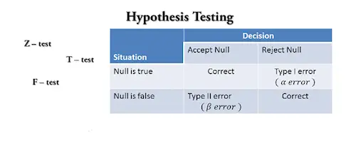
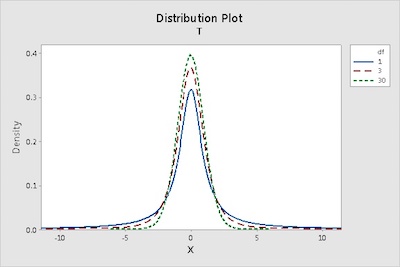
Let’s take a look at the two most common types of test statistics: t-test and F-test.

T-Test And Comparing Means

T-Test-And-Comparing-Means
The hypothesis test is called a two-sample t-test.

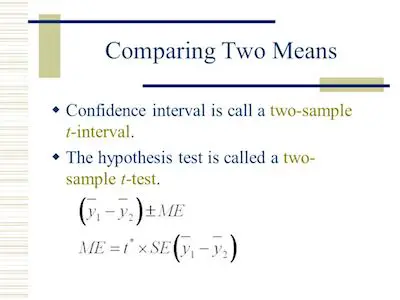
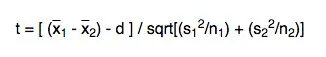
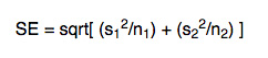
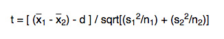
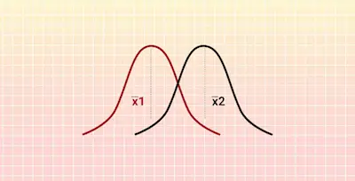
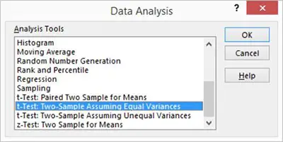
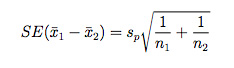
The t-test is a test statistic that compares the means of two different groups. There are a bunch of cases in which you may want to compare group performance such as test scores, clinical trials, or even how happy different types of people are in different places. As you can easily understand, different types of groups and setups call for different types of tests. The type of t-test that you may need depends on the type of sample that you have.

Understanding the basics of probability.

If your two groups are the same size and you are taking a sort of before-and-after experiment, then you will conduct what is called a dependent or Paired Sample t-test. If the two groups are different sizes or you are comparing two separate event means, then you conduct an Independent Sample t-test.

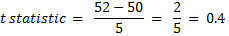
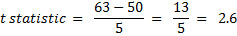
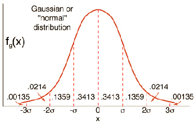
Overall speaking, a t-test is a form of statistical analysis that compares the measured mean to the population mean, or a baseline mean, in terms of standard deviation. Since we are dealing with the same group of people in a before-and-after kind of situation, you want to conduct a dependent t-test. You can think of the without scenario as a baseline to the with scenario.
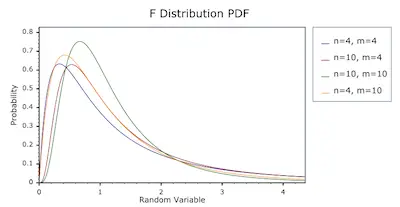
F-Test Statistic

F-Test-Statistic

Sometimes, you want to compare a model that you have calculated to a mean. For example, let’s say that you have calculated a linear regression model. Remember that the mean is also a model that can be used to explain the data.

Learn the measures of position.

The F-Test is a way that you compare the model that you have calculated to the overall mean of the data. Similar to the t-test, if it is higher than a critical value then the model is better at explaining the data than the mean is.

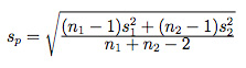
Before we get into the nitty-gritty of the F-test, we need to talk about the sum of squares. Let’s take a look at an example of some data that already has a line of best fit on it.

F-Test-Statistic-graphs

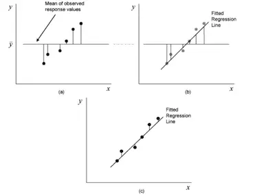
The F-test compares what is called the mean sum of squares for the residuals of the model and the overall mean of the data. Party fact, the residuals are the difference between the actual, or observed, data point and the predicted data point.

Understanding the measures of dispersion.

In the case of graph (a), you are looking at the residuals of the data points and the overall sample mean. In the case of graph (c), you are looking at the residuals of the data points and the model that you calculated from the data. But in graph (b), you are looking at the residuals of the model and the overall sample mean.

The sum of squares is a measure of how the residuals compare to the model or the mean, depending on which one we are working with. 


How To Use The Student’s T Test

As you probably already know, the t distribution which is also known as the Student’s t, is a probability distribution that looks like a bell-shaped curve. This is also known as the normal distribution curve.

Learn more about statistics.

So, ultimately, if you keep sampling from a population in which the null hypothesis is true, then you know that the t distribution shows the long-run probabilities of various t values occurring.

So, what it the t value?

When you want to calculate a t statistic from your data set, you need to use a formula to test a sample mean:

student’s t test

Determine your student t-value here.

In case you discover that the null hypothesis is true, then this means that the sample mean would likely be close to the value you have under your hypothesis. 

Let’s take a look at an example so it can be easier to understand. Imagine that you have a sample mean that is equal to 52, which is close to the hypothesized mean of 50. This means that you would get a numerator will a value near zero. So, you can then conclude that the t statistic will also be close to zero.

t statistic example 1

Whereas, if your sample mean is further away from the hypothesized mean, let’s say 63, the resulting t statistic would be larger.

t statistic example 2

Now, it is the time to see when the t statistic that you just calculated lies on the t distribution. 

Since we are talking about a normal distribution, a bell-shaped curve, the data clusters about the mean. And while the values further away from the mean (i.e. toward the tails of the distribution) are not impossible if the null hypothesis is true, they are unlikely.

So, with the t distribution tables that are available online, you can get the critical values for the t distribution at different levels of significance. 

Check out our free student t-value calculator.

Here’s a screenshot of the table when alpha = 0.05:

table with alpha equal to 5

Notice that the underlying distribution is similar in the different tables. They only vary in what percentage of the distribution is being shown. 

The table we just displayed above tells you that for a specific degree of freedom, what value does 5% of the distribution lie beyond. 

For example, when df (degrees of freedom) = 5, the critical value is 2.57. This means that 5% of the data lies beyond 2.57. So, if your calculated t statistic is equal to or greater than 2.57, you can reject our null hypothesis.

Calculate your student t-value here.

At this point, you need to also take a look at the p-values. In case you don’t know, p-values tell you the probability of obtaining your t statistic, or one more extreme, given the null hypothesis is true. That is, what area of the t distribution lies beyond our calculated t statistic?

t distribution

We already pointed out earlier that for 5 degrees of freedom, the critical t value is 2.57. So, this means that 5% of the distribution lies to the right of the line marking 2.57. 

As you can see above, if your sample mean was 63, you get a calculated t statistic of 2.60. 

The area to the right of this line gives you the p-value; the probability of getting this or more extreme, i.e. what area of the distribution lies to the right of 2.60. In this case, the answer is 2% of the distribution, giving you a p-value of 0.02.


Degrees Of Freedom For T Tests

In case you just started learning statistics or if you already had some classes about it, you probably already heard about degrees of freedom. 

Simply put, in statistics, the degrees of freedom indicate the number of independent values that can vary in an analysis without breaking any constraints. 

degrees of freedom

While this may seem a simple concept (and it is), you need to know that you will need to work with it in many different statistics fields. These include probability distributions, hypothesis tests, and even regression analysis. 

Understanding The Degrees Of Freedom

Before we show you more about the degrees of freedom for t tests, we believe that it is a good idea to tell you more about degrees of freedom in the first place. 

As we already mentioned above, the degrees of freedom are simply the number of independent values that a statistical analysis can estimate. In case this seems very technical, you just need to keep in mind that they are the number of values that can vary freely as you estimate parameters.

Check out our student t-value calculator.

different degrees of freedom

Notice that understanding the degrees of freedom is very simple. So, in case you prefer, you can look at them and keep in mind that they encompass the idea that the amount of independent information that you have may limit the number of parameters that you can estimate. 

In most cases, the degrees of freedom are equal to the difference between your sample size and the number of parameters that you need to calculate during an analysis. Besides, it is important to keep in mind that this is usually a positive whole number. 

As you can easily understand, the degrees of freedom are a mix or a combination of how much data you have and how many parameters you need to estimate. So, ultimately, the degrees of freedom show you how much independent information goes into a parameter estimate. 

When you understand this concept, it is easy to understand that it’s easy to see that you want a lot of information to go into parameter estimates to obtain more precise estimates and more powerful hypothesis tests. So, you want many degrees of freedom.

Calculate the student t-value using our free calculator.

Degrees Of Freedom For T Tests

Degrees Of Freedom For T Tests chart

As you probably already know, t tests are hypothesis tests for the mean and they use the t distribution to determine statistical significance.

When you are using the simple t test or the 1-sample t test as it is also known, you are looking to determine if the difference between the sample mean and the null hypothesis value is statistically significant. 

As you already know, when you have a sample and estimate the mean, you have n – 1 degrees of freedom, where n is the sample size. So, for a 1-sample t test, the degrees of freedom is n – 1.

Need help to determine the student t-value?

Notice that the degrees of freedom define the shape of the t distribution that your t-test uses to calculate the p-value. 

One of the things that is important to notice is that as the degrees of freedom decreases, the t-distribution has thicker tails. This property allows for the greater uncertainty associated with small sample sizes.


When To Use A T Test?

Before we actually answer the question about when to use a t test, we believe that it is important that you know exactly what a t test is. 

Discover everything you need to know about statistics.

What Is A T Test?

t test

Simply put, a t test is a statistical test that was invented by William Sealy Gosset. This test serves to determine if two sample means (averages) or proportions are equal. 

Now that you already understand what a t test is (or at least, you remembered), it is time to know when you should use it. 

When To Use A T Test?

As we already mentioned, a t test is used to compare two proportions or means. So, we can then say that you can use a t test whenever you want to compare means. However, in order to use the t test, some assumptions need to b met. We will take a look at these assumptions below. 

One of the things that you need to keep in mind about the t test is that it is only a good idea to use a t test when the proportions or means are good measures. 

Make sure to use our student t value calculator.

Matched And Unmatched T Tests

It’s important to notice that there are two different forms of the t test: the matched t test and the unmatched t test. So, what’s the difference between the two?

In a matched t test, the two samples are not independent. Just think of the length of people’s left and right feet. These are dependent. After all, when you know the size of your left foot, you immediately know the size of your right foot.

In an unmatched t text, the two samples are independent. This is why this test is also known as the independent t test. As you can easily understand, this means that when you know something about one variable, it won’t affect the other one. For example, the heights of men and women drawn randomly from a population. The truth is that a specific height of a man doesn’t tell you anything about the height of any specific woman. 

Need help to determine the student t value?

T Test: The Assumptions It Needs To Meet

t text assumptions

As we mentioned above, to do a t test, you need to ensure that both samples are independent. Besides, one of the things that you may not know is that both types of t tests assume that the variances of the populations are always equal. 

So, in case you don’t have this last criteria met, you need to know that there are different things you can do to adjust for unequal variances, provided that the sample sizes of the two samples are approximately equal. 

Notice that it is possible that you have two very different variances as well as two very different sample sizes. When this happens, you shouldn’t use the t test.

Discover if you got the right t value.

So, What Do You Use?

In statistics, there are many other tests that can be performed. When you find out that it’s not appropriate to conduct a t test, then you should consider other alternative tests such as the Wilcoxon’s test or the permutation test. 


How To Conduct A T Test In Excel

As you probably already know, a t test can be very useful in statistics. After all, this test allows you to know if there is a difference between the means. In case you don’t know, or simply don’t remember, the bigger the t value, the bigger the difference between the two samples.

Use the best statistic tables. 

While you can do a t test by hand, you should know how to do a t test in excel. After all, this can save you a lot of time. However, you need to understand that when you are working with excel, you can actually make three different t tests:

  • the paired two sample for means
  • the two-sample assuming equal variances
  • the two-sample assuming unequal variances

So, let’s discover how to do a t test in excel.

how-to-do-a-t-test-in-excel

Let’s say that you just collected the data and that you organized the data in your excel spreadsheet. The range A1:A21 contains the first set of values and the B1:B21 contains the second set f values.

Lear more about the two sample t test.

Step #1: Make sure that you choose the “Data Analytics” and then “Data”.

Step #2: Now, you should be able to see the Data Analysis dialog box. So, all you need to do is to pick the t test that you want to make from the Analysis Tools list.

Data-Analysis-dialog-box

As you can see, you’ll be able to choose between:

  • the t-Test: Paired Two-Sample For Means: This is the one that you should choose when you want to make a paired two-sample t test.

  • the t-Test: Two-Sample Assuming Equal Variances: This is the t test that you should choose when you believe that both samples’ means are equal.
  • the t-Test: Two-Sample Assuming Unequal Variances: This is the t test that you need to choose when you want to do a two-sample t test and you believe that the two-sample variances are different.

Step #3: As soon as you decide about the test to perform, just click ok. Let’s say that you chose the second t test. You will then see the following dialog:

second-t-test

While this is just an example, the other dialog windows are very similar so you shouldn’t have any problems filling them in.

Discover everything you need to know about the unpaired t test.  

Step #4: Adding The Inputs:

As you can see, the first fields that you need to fill are the “Variable 1 Range” and the “Variable 2 Range”. All you need to do is to fill in with the ranges that you have for the data. In this case, in the first field you will need to add $A$1:$A$21 and in the second field, $B$1:$B$21. However, to make it easier, you can simply drag the data for the appropriate field directly from the excel spreadsheet.

Check out this simple paired t test example.

The next field that you need to fill is the “Hypothesized Mean Difference”. In this box, you will need to specify whether you believe the means are equal or different. The way that you have to do this is very simple. In case you believe that the means are the same, you just need to add zero (0) in the text box. On the other hand, if you believe they are different, you should add the mean difference.


Next, you need to add the Alpha. This refers to the confidence level that you are using in your t test calculation. The confidence level always varies between 0 and 1. So, you will need to add your own. Please notice that if you don’t add any, the default confidence level will be applied – which is equal to 0.05, which is the same to say that you have a 5% confidence level.

The last area that you need to fill regards to the “Output Options”. And these are simply the place where you want your results to be seen. If you want the results to be displayed in a specific cell, you just need to add it right beside the “Output Range”. Or you can choose one of the other options.

Step #5: Click OK.

As soon as you click OK, the results of the t test will be displayed according to what you specified.


Paired T Test Example

The truth is that doing a paired t test is not as difficult as it may seem when you first look at it. Nevertheless, a paired t test example is always a good way to learn exactly what you need to do.

One of the things that you need to have in mind os that a paired t test is used to compare the means of two populations.

Use the top stats calculators.

The paired t test is very used in many different areas. You can use it to compare different health treatments, to analyze the results of a diagnostic test before and after a specific module, among so many others.

paired-t-test-example

Before we actually show you the paired t test example, let’s see how you need to proceed.

Let’s say that you have a sample of n students. They had to do a diagnostic test before module A and another one after completing it. Our goal is to determine the importance of teaching in the student’ skills and knowledge, evaluated with their scores.

Let’s also consider that:

x – represents the diagnostic test score before Module A

y – represents the diagnostic test score after Module A

In order to start testing the null hypothesis, which is the mean difference is zero, here are the steps you need to take:

Step #1: Calculate the difference between the two observations, before and after the diagnostic test, on each pair:

d = y – x

Learn more about the unpaired t test.

Step #2: Determine the mean difference

Step #3: Determine the standard deviation of the differences. Then, you will need to use this value to calculate the standard error of the mean difference:

standard-error-of-the-mean-difference-formula

Step #4: Determine the t-statistic, by using the following formula:

t-statistic-formula

Please remember that you are testing the null hypothesis. Therefore you need to use the t-distribution with n-1 degrees of freedom.

Step #5: Compare your T value with the tn-1 value that you can check on the t-distribution tables.

What is a 2 sample t test? 

Now, let’s check a practical paired t test example:

Let’s say that we are assuming that we want to measure the results of teaching on students as well and that we already know their scores before and after the Module A was taught. Let’s also consider that we are considering a sample of 20 students. So, n = 20.

Here are the scores that the students had:

StudentPre-Module ScorePost-Module ScoreDifference
11822+4
22125+4
31617+1
42224+2
51916-3
62429+5
71720+3
82123+2
92319-4
101820+2
111415+1
121615-1
131618+2
141926+7
1518180
162024+4
171218+6
182225+3
191519+4
201716-1

In the last column, you can already see the calculations of the differences of the scores for each student. So, all you need to do know is to determine the mean difference, using the formula we provided above.

We can then say that the mean difference is 2.05.

So, by using the values and replacing them in the standard deviation of the differences formula also provided above, you will get:

Sd = 2.837

Now, it’s time to determine the standard error of the mean:

SE(d) = Sd / √n = 2.837 / √20 = 0.634

Discover the top intro statistics books. 

Finally, you will need to perform the t-statistic:

t = 2.05 / 1.634 = 3.231

Please notice that this is the t-statistic calculated for 19 degrees of freedom.

So, by looking at the tables, you can see that you will get a p = 0.004.

With this result, we can say that module A does lead to improvement in the students’ knowledge and skills. In fact, there is even a strong evidence of that.


Understand Unpaired T Test For Two Samples

As you probably already know, a t test is very important in statistics and it tends to be used for a wide variety of subjects and topics. Since it can be used as a very broad test, the truth is that there are some derivations of this test, specifically the unpaired t test.

But what exactly is the unpaired t test?

Simply put, the unpaired t test allows you to compare the means of two different samples. However, in order to perform this test, the values need to follow the Gaussian distribution.

unpaired-t-test

Besides, there are some assumptions that you can withdraw when the unpaired t test was performed:

Check out the most important stats calculators that you need. 

#1: The Two Populations Have The Same Variances:

When you perform an unpaired t test, you assume that both populations have different variances as well as the same standard deviation. While this may not mean much for you so far, you will learn that when populations have different variances this fact can be as important as discovering that they have different means.

#2: The Data Needs To Be Unpaired:

Whenever you have data that is a match or paired, you should use the paired t test instead.

Discover the basic statistics that you need to know about for data science.

#3: You Can Only Compare Two Groups:

One of the most common mistakes statistics students make when they are learning more about t tests and the unpaired t test is to use the unpaired t test multiple times in a row. However, this is something that you should avoid or you’ll be increasing the risk of finding a statistically significant difference by chance. Ultimately, this will make it harder for you to interpret both the statistical significance level as well as the P-value. When you need to make multiple comparisons, a better approach is to use the one-way ANOVA.

So, how do you do an unpaired t test?

As you already know, an unpaired t test is used when you want to compare two population means. Usually, this is how you will see the notations:

n1, n2 – refer to the sample sizes of population 1 and 2, respectively

x¯1, x¯2 – refer to the sample means of population 1 and 2, respectively

s1, s2 – refer to the standard deviation of population 1 and 2 respectively.

Here is how the procedure of carrying out an unpaired t test works:

1. You will be assuming that the null hypothesis states that the two population means are equal. Or:

H0: x¯1 = x¯2

2. The first thing that you will need to do is to determine the difference between the two sample means, or:

x¯1 – x¯2

3. Next, you will need to take a closer look at the standard deviation. However, you won’t be looking at the standard deviation of each one of the samples individually. Instead, you will need to calculate the pooled standard deviation:

pooled-standard-deviation-formula

4. In this step, you will need to determine the standard error of the difference between the two means. So, you will need to use the following formula:

standard-error-of-the-difference-between-the-two-means

5. Now, it is finally time to determine the t-statistic. You can easily do it by using the formula:

t = ( x¯1 – x¯2 ) / SE ( x¯1 – x¯2 )

Please note that when you are testing the null hypothesis, you already know that the t will follow a t-distribution with n1 + n2 – 2 degrees of freedom.

Learn more about statistical questions. 

6. Finally, you will need to use the t-distribution tables to compare the value of the t that you got with the tn1+n2−2 distribution. This will give you the p-value for the unpaired t test.

As you ca see, the unpaired t test is easily done. While it includes multiple steps, it is very simple to perform. Nevertheless, if you are seeing all this information for the first time, it may be a bit harder to understand this test without any values. So, let’s take a look at an example of an unpaired t test.

Unpaired T Test – Practical Example:

Let’s say that a company decided to do a study about the number of calories included in the hotdog meat. The truth is that not all hotdog meat is the same and there are some brands that use beef and others that use poultry. So, as you can imagine, the calories contained in both dogs should be different.

After processing the data, the company presented the following data:


GroupSample SizeSample MeanSample Standard Deviation
Beef20156.8522.64
Poultry17122.4725.48

Since we believe these values can follow the Gaussian distribution, we can then proceed with the unpaired t test that we just described above.

1. Let’s start by determining the difference of the means: x¯1 – x¯2

In this case, x¯1 – x¯2 = 156.85 − 122.47 = 34.38

2. Now, it is time to determine the pooled standard deviation. By replacing the numbers of the table into the formula directly:

Sp = √ [[ (n1-1)s1^2 + (n2-1)s2^2 ] / n1 + n2 – 2] = √ [[ (19)22.64^2 + (16)25.48^2 ] / 35] = 23.98

3. Now, in order to determine SE(¯x1 − x¯2):

SE(¯x1 − x¯2) = Sp√ [ (1/n1) + (1/n2) ] = 23.98√[ (1/20)+(1/17) ] = 7.91

What exactly is a statistical question?

4. Finally, you can now calculate the value of the T:

t = ( x¯1 – x¯2 ) / SE ( x¯1 – x¯2 )

t = 34.38/7.91

5. By checking the tables of the t-distribution with 35 degrees of freedom, you will easily discover that p<0.001. So, we can say, almost for sure or with a high degree of certainty, that poultry dogs have fewer calories than beef hotdogs.

Even if you are just learning statistics and the unpaired t test for the first time, we believe that you now have a good knowledge about this specific test and that you won’t have any problems with the procedure.


Two Sample T Test Explained

Before we even start talking about a 2 sample t test, it is important that you understand what a t-test is and what is its purpose in statistics. Simply put, a t test is a hypothesis test that allows you to compare means.

So, based on this simple definition, you can easily understand that a 2 sample t test is another hypothesis test that served to compare means but with the difference that you have two random data samples.

Take a look at the best statistics calculators.


2-sample-t-test
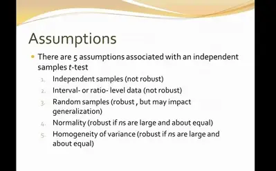
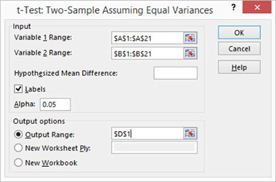
One of the main reasons why researchers and statistics tend to use the 2 sample t test is when they need to evaluate the means of two different groups or variables and understand if these means differ or are the same. For example, the 2 sample t test is very used to determine the effects of receiving a treatment of males versus females.

One of the main advantages of using a 2 sample t test is the fact that you can use it with small and large data samples.

Now that you already understand what a 2 sample t test is and what its purpose is, it is time to see it in action. The reality is that there are two common applications for the 2 sample t test:

Learn more about quantitative reasoning questions and answers.

#1: Using The 2 Sample T Test To Determine That The Means Are Equal:

When you are looking to use this test to see if the means of the two samples of data you collected are the same, you need to follow the next steps:

Step 1. Define The Hypothesis:

The following table shows three different of hypothesis: three nulls and three alternatives.

SetNull HypothesisAlternative HypothesisNumber of Tails
1μ1 – μ2 = dμ1 – μ2 ≠ d2
2μ1 – μ2 > dμ1 – μ2 < d1
3μ1 – μ2 < dμ1 – μ2 > d1

As you can see, each one of this hypothesis shows the difference (d) between the mean of the two populations – μ1, the mean of population 1, and μ2 the mean of the population 2.

Step 2. Determine The Significance Level:

While you can use any value between 0 and 1, most researchers tend to use0.10, 0.05 or 0.01 as the significance level.

Step 3. Determining The Degrees Of Freedom (DF):

While you may see that the degrees of freedom can be determined in a simpler way, in order to be more exact, you should use the following formula:

DF = (s1^2/n1 + s2^2/n2)^2 / { [ (s1^2 / n1)^2 / (n1 – 1) ] + [ (s2^2 / n2)^2 / (n2 – 1) ] }

When you are determining the degrees of freedom using this formula, you may not get an integer. In this case, you need to make sure that you round it off to the nearest whole number.

Looking for the best introductory statistics books?

Step 4. The Test Statistic:

In order to compute the test statistic, you will need to use the following formula:

test-statistic

test-statistic-2

d – refers to the hypothesized difference between the means of the population

s1 – refers to the standard deviation of sample 1

s2 – refers to the standard deviation of sample 2

n1 – refers to the size of sample 1

n2 – refers to the size of sample 2

Step 5. Determine The P Value:

In case you don’t know, the P-value is just the probability of observing a specific sample statistic as extreme as the test statistic.

Step 6. Evaluating The Results:

The result of the test will come from the comparison between the P-value with the significance level. So, in case the P-value is less than the significance level, the null hypothesis is rejected.

#2: Using The 2 Sample T Test To Determine The Difference Between Means:

In this case, you need to make sure that you comply with the following rules so that you know that you can perform a 2 sample t test:

  • the samples are independent
  • the sampling method that was used for each sample was the simple random sampling
  • the population distribution is normal
  • the population needs to be at least 20 times larger when compared with its sample
  • the sampling distribution seems to be approximately normal.

If all these conditions are met, you can start the 2 sample t test by following the next steps:

Step 1. State The Hypothesis:

On the following table, you can see three different sets of data where you have both the null and alternate hypothesis. Please notice that this is a similar table to the one we showed before.

SetNull HypothesisAlternative HypothesisNumber of Tails
1μ1 – μ2 = dμ1 – μ2 ≠ d2
2μ1 – μ2 > dμ1 – μ2 < d1
3μ1 – μ2 < dμ1 – μ2 > d1

In this case, you can see that the set 1 and the sets 2 and 3 are different. This is why we will need to to use a two-tailed test for the set 1 and the next 2 sets need to be tested using a one-tailed test.

When we want to have the null hypothesis to say that the means of the different populations are the same, which is the same as saying that d=0, then you can have the null and alternate hypothesis like this:

Ho: μ1 = μ2

Ha: μ1 ≠ μ2

Step 2. Defining The Analysis Plan:

In order to have your analysis plan all set, you need to ensure that you considered several elements:

  • The Significance Level, which, again, you should use 0.10, 0.05 or 0.01.
  • The Test Method, which you will need to use the 2 sample t test.

Learn how to calculate the P value from Z. 

Step 3. Analysis Of Sample Data:

The analysis of sample data includes discovering the standard error, the degrees of freedom, determining the test statistic, and finally determining the P-value that is associated with the test statistic. Here’s how it is done:

  • Standard Error: Just use the following formula:

standard-error

where,

s1 – is the standard deviation of sample 1

s2 – is the standard deviation of sample 2

n1 – is the size of sample 1

n2 – is the size of sample 2

  • Degrees Of Freedom: You just need to use the formula above.
  • Test Statistic: Just use the following equation of the t statistic (t):

test-statistic

test-statistic-2

  • P-Value.

Step 4. Interpreting The Results:

In order to interpret the results, you will need to compare the P-value with the significance level. In case the P-value is inferior, which is what happens most of the times, you will reject the null hypothesis.

The last concept that you need to know about when we are talking about a 2 sample t test is the paired t test formula concept. Simply put, while you will use the 2 sample t test when you have two completely different populations, you will have to use the paired t test when the samples that you have are connected in some way.