How To Interpret Regression Coefficients
When you are learning statistics, you are probably already familiar with linear regression. After all, it is one of the most popular statistical techniques. However, while it seems pretty simple and obvious, the reality is that interpreting regression coefficients of some models may be difficult.
Discover all the statistics calculators you can use.
How To Interpret Regression Coefficients
To help you overcome these difficulties in interpreting regression coefficients, let’s try to interpret the coefficients of a continuous and a categorical variable.
Notice that while we are using the linear regression, you can apply the same basics to interpret the coefficients from any other regression model without interactions.
Learn more about the binomial distribution.
Linear Regression
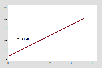
As you probably already know, a linear regression model with two predictor variables can be expressed with the following equation:
Y = B0 + B1*X1 + B2*X2 + e
The variables in the model are:
- Y, the response variable;
- X1, the first predictor variable;
- X2, the second predictor variable; and
- e, the residual error, which is an unmeasured variable.
The parameters in the model are:
- B0, the Y-intercept;
- B1, the first regression coefficient; and
- B2, the second regression coefficient.
One simple example would be a model of the height of a shrub (Y) based on the amount of bacteria in the soil (X1) and whether the plant is located in partial or full sun (X2).
Let’s consider that the height is measured in cm, bacteria is measured in thousand per ml of soil, and the type of sun = 0 if the plant is in partial sun and type of sun = 1 if the plant is in full sun.
Imagine that the regression equation was estimated as follows:
Y = 42 + 2.3*X1 + 11*X2
Discover the differences between descriptive and inferential statistics.
Interpreting The Intercept
B0, the Y-intercept, can be interpreted as the value you would predict for Y if both X1 = 0 and X2 = 0.
This means that we would expect an average height of 42 cm for shrubs in partial sun with no bacteria in the soil. But it is important to notice that this is only a meaningful interpretation in case both X1 and X2 can be 0. Besides, the data set also needs to include values for X1 and X2 that were near 0.
In our example, it is easy to see that X2 sometimes is 0, but if X1, our bacteria level, never comes close to 0, then our intercept has no real interpretation.
Looking to know more about confidence intervals?
Interpretation Of Coefficients Of Continuous Predictor Variables
Since X1 is a continuous variable, B1 represents the difference in the predicted value of Y for each one-unit difference in X1, if X2 remains constant. So, as you can easily understand, if X1 differed by one unit (and X2 did not differ) Y will differ by B1 units, on average.
Looking back at our example, shrubs with a 5000 bacteria count would, on average, be 2.3 cm taller than those with a 4000/ml bacteria count, which likewise would be about 2.3 cm taller than those with 3000/ml bacteria, as long as they were in the same type of sun.
Interpretation Of Coefficients Of Categorical Predictor Variables
Now, if we take a look at B2, it can be interpreted as the difference in the predicted value in Y for each one-unit difference in X2 if X1 remains constant. However, since X2 is a categorical variable coded as 0 or 1, a one unit difference represents switching from one category to the other. We can then state that B2 is the average difference in Y between the category for which X2 = 0 (the reference group) and the category for which X2 = 1 (the comparison group).
So compared to shrubs that were in partial sun, we would expect shrubs in full sun to be 11 cm taller, on average, at the same level of soil bacteria.