Category : Regressions

What is Logistic Regression?

When you are conducting a study, there’s nothing better than having all your data nice and straight. After all, you know that when this happens, it is easier to predict outcomes. However, this doesn’t always happen. 

Discover the best online statistics calculators.

logistic-regression

The reality is that sometimes, you want to know how likely something happens and not the actual outcome. So, you need to look at logistic regression.

What is Logistic Regression?

As you probably remember, variables can be either categorical or continuous. Categorical variables are the ones that exist as some sort of discrete unit like multiple choice answers. On the other hand, continuous variables are the ones that exist on some scale like gas mileage or height. 

As you can easily understand, each type of variable has a particular type of statistics linked with them due to their nature. 

Understanding the difference between correlation and linear regression.

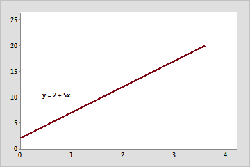
In the case of linear regression, you deal with continuous variables. This way, you can analyze the data and predict an outcome based on a scale. However, in what concerns to categorical variables, there are no traditional scales or lines. So, this means you can’t use linear regression. 

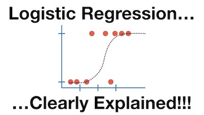
So, when this happens, the first thing you need to look at is binary logistic regression. Let’s take a look at a more practical example. Imagine that you just asked some people if they think the temperature (in Fahrenheit) is too hot. Their answers are expressed in the chart below:

temperature-in-Fahrenheit-graph

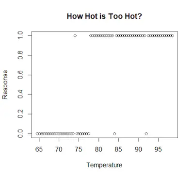
As you can see, the data isn’t a normal scatter plot. You can see that the data points aren’t all over the place – they are focused on either 1 or 0 because these were the answers people have to choose from. 

Discover how to perform a simple regression analysis.

This means you can’t calculate the typical line as you would for linear regression because there is no “sort of” response.

Instead, you need to calculate the probability of a person responding either 1 or 0. That is what binary logistic regression is for. We use it to calculate the chance of a person responding to one of two choices.

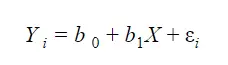
The general model for binary logistic regression is:
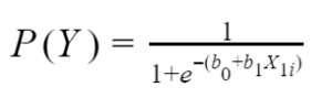
general-model-for-binary-logistic-regression

Where:

  • P(Y) means that we are calculating the probability of an outcome of 1 occurring. 
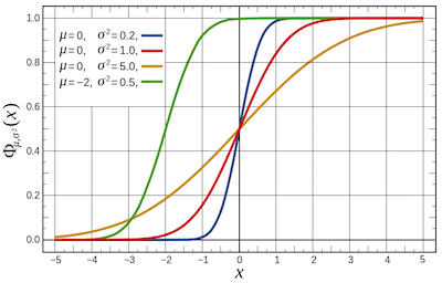
  • e shows the use of logarithmic functions that create a line of best fit for the data.

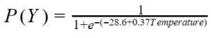
So, after running the analysis, your model looks like this:

after-running-the-analysis

Is Your Model Any Good?

One of the things that you always need to keep in mind about logistic regression is that this type of model can’t be interpreted as a linear regression model using R2. 

The truth is that with the logistic regression, you are interested in the probability of an outcome and not in the actual outcome. Therefore, you need to consider the likelihood of an outcome. This is called log-likelihood.

Learn how to interpret regression coefficients.

Simply put, the log-likelihood refers to adding the probability of the predicted outcome to the probability of the actual outcome so that you can get a sense of how well our model explains all the probability of the event occurring.


How To Perform A Simple Regression Analysis

When you have data, most of the time, you should start to analyze it using a graph or some sort of linear regression. However, as soon as you realize, you get an equation. And this is exactly where simple regression analysis comes in. 

simple regression analysis

Discover the best online statistics calculators.

Looking Into The Simple Regression Analysis

Before we take a deeper look at the simple regression analysis, we believe that we should start by reviewing what makes a regression. 

The truth is that simple regression analysis simply refers to the interpretation and use of the regression equation. In case you don’t remember, this is how it looks like:

Learn how to deal with missing data in statistics.

regression equation

The Yi represents the dependent variable in your equation. This refers to the effect or outcome that we are interested in. Xi represents the independent variable and this is the variable that we think predicts the outcome.

In what concerns to the other things, this is where things become more interesting. The b1 represents the actual relationship between the independent and dependent variable. Now, the b0 is more of a theoretical term instead of a practical one. It technically means that when the independent variable is equal to zero, then the dependent variable is equal to b0. 

The last part of the equation is εi. This is the error term or the range of wrongness associated with your equation. However, the error term is usually combined with b0 to make the equation a little easier to use.

Learn more about the binomial distribution.

Simple Regression Analysis

simple regression analysis graph

If you take a look at the above graph, you can see a line surrounded by a lot of dots. Each dot represents a data point with an independent variable and a dependent variable. So, using the equation

Linear regression equation

You can come up with just a line that ends up representing the data. 

One of the things that you need to keep in mind is that this line isn’t a perfect fit for the data. Nevertheless, it is still a good prediction. And this is exactly what the regression analysis does: it predicts a dependent based on the independent variable. 

Understand the difference between descriptive and inferential statistics.

How Good Is The Prediction?

When you are calculating the regression equation for the data set that you have, you need to ensure that you also calculate the correlation coefficient. 

Simply put, the correlation coefficient is a value between -1 and +1 which represents the strength of the regression equation’s ability to predict an outcome. 

The closer the correlation coefficient is to 1 (either negative or positive), the stronger the relationship, with 1 being a perfect prediction. The formula is:

correlation coefficient formula

Notice that the correlation coefficient is different from the coefficient of determination, r2. Simply put, the coefficient of determination is more explanatory since it tells you how much of the variability in the outcome is due to the variability in the predictor.

Overall speaking, a high coefficient of determination means that most of the variance of the model is explained by the independent and dependent variables. On the other hand, a low coefficient of determination means that there is a lot of variance that the model doesn’t explain.


How To Interpret Regression Coefficients

When you are learning statistics, you are probably already familiar with linear regression. After all, it is one of the most popular statistical techniques. However, while it seems pretty simple and obvious, the reality is that interpreting regression coefficients of some models may be difficult. 

Discover all the statistics calculators you can use.

How To Interpret Regression Coefficients

regression-coefficients

To help you overcome these difficulties in interpreting regression coefficients, let’s try to interpret the coefficients of a continuous and a categorical variable. 

Notice that while we are using the linear regression, you can apply the same basics to interpret the coefficients from any other regression model without interactions. 

Learn more about the binomial distribution.

Linear Regression

Linear-Regression

As you probably already know, a linear regression model with two predictor variables can be expressed with the following equation:

Y = B0 + B1*X1 + B2*X2 + e

The variables in the model are:

  • Y, the response variable;
  • X1, the first predictor variable;
  • X2, the second predictor variable; and
  • e, the residual error, which is an unmeasured variable.

The parameters in the model are:

  • B0, the Y-intercept;
  • B1, the first regression coefficient; and
  • B2, the second regression coefficient.

One simple example would be a model of the height of a shrub (Y) based on the amount of bacteria in the soil (X1) and whether the plant is located in partial or full sun (X2).

Let’s consider that the height is measured in cm, bacteria is measured in thousand per ml of soil, and the type of sun = 0 if the plant is in partial sun and type of sun = 1 if the plant is in full sun.

Imagine that the regression equation was estimated as follows:

Y = 42 + 2.3*X1 + 11*X2

Discover the differences between descriptive and inferential statistics.

Interpreting The Intercept

Interpreting-The-Intercept

B0, the Y-intercept, can be interpreted as the value you would predict for Y if both X1 = 0 and X2 = 0.

This means that we would expect an average height of 42 cm for shrubs in partial sun with no bacteria in the soil. But it is important to notice that this is only a meaningful interpretation in case both X1 and X2 can be 0. Besides, the data set also needs to include values for X1 and X2 that were near 0.

In our example, it is easy to see that X2 sometimes is 0, but if X1, our bacteria level, never comes close to 0, then our intercept has no real interpretation.

Looking to know more about confidence intervals?

Interpretation Of Coefficients Of Continuous Predictor Variables

Since X1 is a continuous variable, B1 represents the difference in the predicted value of Y for each one-unit difference in X1, if X2 remains constant. So, as you can easily understand, if X1 differed by one unit (and X2 did not differ) Y will differ by B1 units, on average.

Looking back at our example, shrubs with a 5000 bacteria count would, on average, be 2.3 cm taller than those with a 4000/ml bacteria count, which likewise would be about 2.3 cm taller than those with 3000/ml bacteria, as long as they were in the same type of sun.

Interpretation Of Coefficients Of Categorical Predictor Variables

Now, if we take a look at B2, it can be interpreted as the difference in the predicted value in Y for each one-unit difference in X2 if X1 remains constant. However, since X2 is a categorical variable coded as 0 or 1, a one unit difference represents switching from one category to the other. We can then state that B2 is the average difference in Y between the category for which X2 = 0 (the reference group) and the category for which X2 = 1 (the comparison group).

So compared to shrubs that were in partial sun, we would expect shrubs in full sun to be 11 cm taller, on average, at the same level of soil bacteria.


The Distribution of Independent Variables in Regression Models

When you are using regression models, it is normal that you use some distribution assumptions. However, there is one that can’t have any assumptions – the one that refers to independent variables. But why?

The reality is that if you think about it, this makes perfect sense. The reality is that regression models are directional. So, this means that in a correlation, there is no evident direction since Y and X are interchangeable. So, even if you switch the variables, you would end up with the same correlation coefficient. 

regression models

Use the best statistics calculators.

Nevertheless, it is important to keep in mind that regression is a model about the outcome variable. So, what predicts its value and how well does it predict it? And how much of its variance can be explained by its predictors? If you notice, we are posing questions that are all about the outcome. 

One of the things that you should keep in mind about regression models is the fact that the outcome variable is considered a random variable. So, as you can easily understand, this means that while you can explain or even predict some of its variation you can’t really explain all of it. After all, it is subject to some sort of randomness that affects its value in any particular situation. 

In what concerns predictor variables, this isn’t true. After all, when we are talking about predictor variables, we are talking about variables that assume to have no random process. So, there are absolutely no assumptions about the distribution of predictor variables. Besides, they don’t have to be normally distributed, continuous, or even symmetric. But you still need to be able to interpret their coefficients. 

Discover how to calculate the p-value for a student t-test.

Analyzing The Distribution of Independent Variables in Regression Models

Distribution of Independent Variables

#1: You need to have a one-unit difference in X. In case X is numeric and continuous, then a one-unit difference in X makes perfect sense. On the other hand, if X is numeric but discrete, then a a one-unit difference still makes sense.

If X is nominal categorical, a one-unit difference doesn’t make much sense on its own. A simple example of this variable is Gender. In case you code the two categories of Gender to be one unit apart from each other, as is done in dummy coding, or one unit apart from the grand mean, as is done in effect coding, you can force the coefficient to make sense.

But what if X is ordinal–ordered categories? There is no clever coding scheme that can preserve the order, but not treat all the one-unit differences as equivalent. So while there are no assumptions that X are not ordinal, there is no way to interpret coefficients in a meaningful way. So you are left with two options–lose the order and treat it as nominal or assume that the one-unit differences are equivalent and treat it as numeric.

statistical models

Discover how to calculate the t-statistic and degrees of freedom.

#2: While the structure of Y is different for different types of regression models, as long as you take that structure into account, the interpretation of coefficients is the same. This means that although you need to have to take the structure of Y into account, a dummy variable or a quadratic term works the same way in any regression model.

#3: The unit in which X is measured matters. This might be useful to conduct a linear transformation on X to change its scaling. 

Learn how to calculate the two-tailed area under the standard normal distribution.

#4: The other terms in the model matter. Some coefficients are interpretable only when the model contains other terms. For example, interpretations aren’t interpretable without the terms that make them up (lower-order terms). And including an interaction changes the meaning of those lower-order terms from main effects to marginal effects.


Steps to Take When Your Regression Results Look Wrong

When you are doing statistical analysis, sometimes you stop wondering if your results can actually be correct. The truth is that while you took all the necessary steps and you are interpreting them, it seems that they just don’t make sense. No matter if you are thinking about the results using logic or theories, they just look wrong. 

regression results

Discover all the stats calculators you need.

The truth is that the first feeling you tend to experience on these occasions is panic. However, there’s no need to feeling this way. In fact, while there are many possible causes of incorrect results, there are some steps that you can take that will help you discover what you did wrong and how you can correct it. 

Steps to Take When Your Regression Results Look Wrong

#1: Errors In Data Coding And Entry:

One of the most common errors that you may commit when you are doing regressions is regarded with data coding and entry. 

The truth is that you may forget to reverse code the negatively-worded items on a scale, for example. And while they may not be that important, you will see them when you place them in the wrong place if you look at bivariate graphs.

Check out our Z-score calculator.

#2: Misinterpretations:

Misinterpretations

One of the things that tend to happen frequently is that sometimes, your results aren’t wrong. You’re interpreting or reading them the wrong way. 

Notice that while some misinterpretations come from software defaults, others come from the way the statistics are calculated. And on this kind of error, regression coefficients may be a bit tricky. After all, they change meaning depending on other terms in the model. 

For example, with an interaction term in a regression model, coefficients of the component terms are not main effects, as they are without the interaction. So including an interaction can easily reverse or otherwise drastically change what looks like the same coefficient.

Looking for a binomial probability calculator?

#3: Misspecifying The Model:

Misspecifying The Model

Another common factor that may lead to regression results looking wrong is that you may not be using the best model for the data you have. So, in this case, your results may look wrong because they’re not accurate. Maybe you need to use a different type of model for your design and variables or there might be some effects that you didn’t include such as important control variables, non-linear effects, or interactions. 

#4: Bigger Data Issues:

Bigger Data Issues

You already know that when you are doing statistical analysis you need to use high-quality data. However, you may have an issue with missing data and when you are using a software in multivariate analyses, this may lead to getting a lot of data getting dropped even if the percentage of missing data is small on any one variable. 

Check out our student t-value calculator.

Steps to Take When Your Regression Results Look Wrong

So, how can you know what problem you are having? 

The truth is that you just need to follow some steps in order to discover what you should do:

#1:  Run univariate and bivariate descriptive statistics and graphs. 

#2: Read output and syntax carefully. 

#3: Check model assumptions and diagnose data issues like multicollinearity and missing data. Most model misspecifications will appear in model diagnostics.

Finally, consider the possibility that the unexpected result is correct. If you’ve gone through all the diagnoses thoroughly and you can be confident there aren’t any errors, accept the unexpected results. They’re often more interesting.