If you just decided to start studying statistics, then you need to know that there are some statistics basics that you need to be aware off. The truth is that these statistics basics that we are about to show you give you the basis of this new area and will be helpful as you’re now starting.
Discover everything you need to know about statistics.
The reality is that statistics os a powerful tool when you are doing data analysis. After all, it allows you to get a lot of information and, sometimes, you are simply using simple charts and graphs. While a simple bar chart may deliver a high-level of information, the truth is that with statistics, you can get a more information-driven and target way. Ultimately, math helps you get to concrete answers and conclusions to the question that you are studying.
With statistics, you get a deeper insight into how your data is structured and then, based on that structure, how you can apply different techniques to get even more information.
So, now that you already know that you need to learn some statistics basics, it is time to get started.
Basics Of Statistics
One of the things that you need to understand about basics in statistics is that there are many different concepts and formulas that you need to always keep in mind. But don’t worry because we are going to take a look at each one of them.
Statistics Basic Concepts
There’s no question that when you are looking at data that you collected and trying to get more information out of it, you will need to use some statistical features such as bias, variance, mean, median, percentiles, among others.
If you take a look at the above image, you will see different statistics basic concepts that are important when you are learning statistics.
As you can see, the line in the middle is called the median value of the data. Ultimately, the median is used over the mean because it is more robust to outlier values. Then, you can see the quartiles. The first one is the 25th percentile which means that 25% of the points in the data fall below that value. On the opposite side, you have the third quartile which is the 75th percentile. This means that 75% of the points in the data fall below that value. Last but not least, you can also see the min and max values that represent the upper and lower ends of our data range.
Check out our standard error calculator.
Besides, these simple basics in statistics, there is another one that is known as the three Ms:
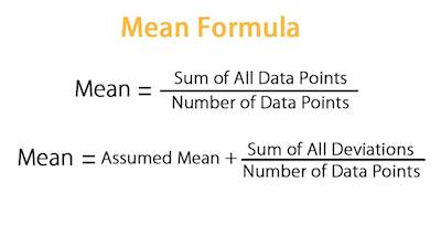
#1: Mean:
The mean is just the average result of an experiment, test, survey, or quiz. So, how can you calculate it?
Here’s an example. Let’s say that you discovered the heights of 5 different people: 5 feet 6 inches, 5 feet 7 inches, 5 feet 10 inches, 5 feet 8 inches, 5 feet 8 inches.
In order to determine the mean, you need to sum up all the heights and then divide the sum total by the number of heights that you discovered. So, in this case:
Mean = (5 feet 6 inches + 5 feet 7 inches + 5 feet 10 inches + 5 feet 8 inches + 5 feet 8 inches) / 5
Mean = 339 inches / 5
Mean = 67.8 inches or 5 feet 7.8 inches
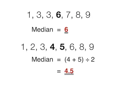
#2: Median:
Median is the middle value of your data. So, as you can imagine, you need to calculate the median differently in case you have an odd amount of values or an even amount of values. Let’s take a look at each one of these cases:
Let’s take the previous example we used to calculate the mean above. In case you don’t remember, you had collected the heights of 5 people: 5 feet 6 inches, 5 feet 7 inches, 5 feet 10 inches, 5 feet 8 inches, 5 feet 8 inches.
To calculate the median, you need to order the numbers from the smallest to the largest first:
5 feet 6 inches, 5 feet 7 inches, 5 feet 8 inches, 5 feet 8 inches, 5 feet 10 inches
As you can see, the value in the middle is 5 feet 8 inches which is also the median.
Learn more about the standard deviation.
Let’s take another example of data. Imagine that you got the following values when you collected your data: 7, 2, 43, 16, 11, 5.
The first thing that you need to do to determine the median is to, again, line up the values in order from the smallest to the largest:
2, 5, 7, 11, 16, 43
And now you have 2 values in the middle – 7 and 11. To determine the median, you will need to calculate the mean between these two values:
Median = (7 + 11) / 2
Median = 9
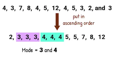
#3: Mode:
The mode is just the most common result that appears in your data set. Let’s use the same heights’ example once again: 5 feet 6 inches, 5 feet 7 inches, 5 feet 10 inches, 5 feet 8 inches, 5 feet 8 inches.
So, to determine the mode, you can put these values in order to make it easier to find the most common value in the data:
5 feet 6 inches, 5 feet 7 inches, 5 feet 8 inches, 5 feet 8 inches, 5 feet 10 inches
As you can see, the only value that repeats is 5 feet 8 inches – it occurs two times.
Looking to calculate the standard error of the mean?
Variance
In statistics, another important concept that you need to understand is variance. Simply put, variance is just the spread of a data set. So, you can say that it is a measurement that is used to identify how far each number in the data set is from the mean.
One of the things that you need to know about variance is that this is an important concept especially when you want to calculate probabilities of future events. The reality is that it is a great way to find all the possible values and likelihoods that a random variable can take within a specific range.
Some of the implications of the variance concept that you should keep in mind include:
- The larger the variance, the more spread is in the data set.
- A large variance means that there are more values far from the mean and far from each other.
- A small variance means that the values in your data set are closer together in value.
- When you have a variance that is equal to zero, this means that all of the values within your data set are identical.
- All variances that are not equal to zero are positive numbers.
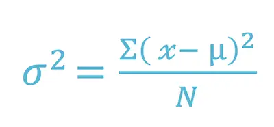
Now that you understand what variance is, you need to know how to calculate it. Simply put, the variance is the difference between each number in the data set and the mean, squaring the difference to make it a positive number, and then dividing it by the number of values on your data set. Here’s the formula:
Where:
X = individual data value
u = the mean of the values
N = total number of data values in your data set.
One of the things that is worth noting is that when you are calculating a sample variance to estimate a population variance, the denominator of the variance equation becomes N – 1. This removes bias from the estimation, as it prohibits the researcher from underestimating the population variance.
One of the main advantages of variance is the fact that it treats all deviations from the mean of the data set in a similar way, no matter the direction. The main disadvantage of using the variance is the fact that it gives added weight to values that are far from the mean (outliers). And when you square these numbers, you may get skewed interpretations of the data set as a whole.
Use our standard error calculator to confirm your results.
Covariance
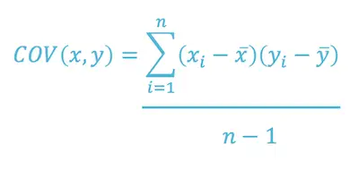
Among the statistics basics formulas, there is another one that is especially important – covariance. But before we get to the formula, you need to understand what covariance is.
Simply put, covariance shows you how two variables are related to one another. So, more technically, covariance refers to the measure of how two random variables in a data set will change together.
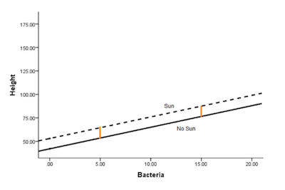
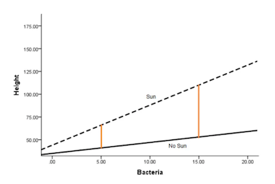
- When you have a positive covariance, this means that the two variables are positively related which is the same as saying that they move in the same direction.
- When you have a negative covariance, this means that the two variables are inversely related which is the same as saying that they move in opposite directions.
Here’s the covariance formula:
Where:
X = represents the independent variable
Y = represents the dependent variable
N = represents the number of data points in the sample
X-Bar = represents the mean of the X
Y-Bar = represents the mean of the dependent variable Y
Bottom Line
As you can see, these basic statistical terms are very simple to understand and you shouldn’t have any difficulties in putting them into practice. However, these basic concepts and formulas are extremely important since they are the basis of statistics.