Category : Uncategorized

Before we even start talking about a 2 sample t test, it is important that you understand what a t-test is and what is its purpose in statistics. Simply put, a t test is a hypothesis test that allows you to compare means.

So, based on this simple definition, you can easily understand that a 2 sample t test is another hypothesis test that served to compare means but with the difference that you have two random data samples.

Take a look at the best statistics calculators.

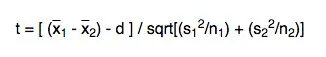
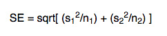
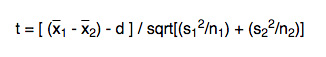
One of the main reasons why researchers and statistics tend to use the 2 sample t test is when they need to evaluate the means of two different groups or variables and understand if these means differ or are the same. For example, the 2 sample t test is very used to determine the effects of receiving a treatment of males versus females.

One of the main advantages of using a 2 sample t test is the fact that you can use it with small and large data samples.

Now that you already understand what a 2 sample t test is and what its purpose is, it is time to see it in action. The reality is that there are two common applications for the 2 sample t test:

Learn more about quantitative reasoning questions and answers.

#1: Using The 2 Sample T Test To Determine That The Means Are Equal:

When you are looking to use this test to see if the means of the two samples of data you collected are the same, you need to follow the next steps:

Step 1. Define The Hypothesis:

The following table shows three different of hypothesis: three nulls and three alternatives.

As you can see, each one of this hypothesis shows the difference (d) between the mean of the two populations – μ1, the mean of population 1, and μ2 the mean of the population 2.

Step 2. Determine The Significance Level:

While you can use any value between 0 and 1, most researchers tend to use0.10, 0.05 or 0.01 as the significance level.

Step 3. Determining The Degrees Of Freedom (DF):

While you may see that the degrees of freedom can be determined in a simpler way, in order to be more exact, you should use the following formula:

DF = (s1^2/n1 + s2^2/n2)^2 / { [ (s1^2 / n1)^2 / (n1 – 1) ] + [ (s2^2 / n2)^2 / (n2 – 1) ] }

When you are determining the degrees of freedom using this formula, you may not get an integer. In this case, you need to make sure that you round it off to the nearest whole number.

Looking for the best introductory statistics books?

Step 4. The Test Statistic:

In order to compute the test statistic, you will need to use the following formula:

d – refers to the hypothesized difference between the means of the population

s1 – refers to the standard deviation of sample 1

s2 – refers to the standard deviation of sample 2

n1 – refers to the size of sample 1

n2 – refers to the size of sample 2

Step 5. Determine The P Value:

In case you don’t know, the P-value is just the probability of observing a specific sample statistic as extreme as the test statistic.

Step 6. Evaluating The Results:

The result of the test will come from the comparison between the P-value with the significance level. So, in case the P-value is less than the significance level, the null hypothesis is rejected.

#2: Using The 2 Sample T Test To Determine The Difference Between Means:

In this case, you need to make sure that you comply with the following rules so that you know that you can perform a 2 sample t test:

• the samples are independent
• the sampling method that was used for each sample was the simple random sampling
• the population distribution is normal
• the population needs to be at least 20 times larger when compared with its sample
• the sampling distribution seems to be approximately normal.

If all these conditions are met, you can start the 2 sample t test by following the next steps:

Step 1. State The Hypothesis:

On the following table, you can see three different sets of data where you have both the null and alternate hypothesis. Please notice that this is a similar table to the one we showed before.

In this case, you can see that the set 1 and the sets 2 and 3 are different. This is why we will need to to use a two-tailed test for the set 1 and the next 2 sets need to be tested using a one-tailed test.

When we want to have the null hypothesis to say that the means of the different populations are the same, which is the same as saying that d=0, then you can have the null and alternate hypothesis like this:

Ho: μ1 = μ2

Ha: μ1 ≠ μ2

Step 2. Defining The Analysis Plan:

In order to have your analysis plan all set, you need to ensure that you considered several elements:

• The Significance Level, which, again, you should use 0.10, 0.05 or 0.01.
• The Test Method, which you will need to use the 2 sample t test.

Learn how to calculate the P value from Z. 

Step 3. Analysis Of Sample Data:

The analysis of sample data includes discovering the standard error, the degrees of freedom, determining the test statistic, and finally determining the P-value that is associated with the test statistic. Here’s how it is done:

• Standard Error: Just use the following formula:

where,

s1 – is the standard deviation of sample 1

s2 – is the standard deviation of sample 2

n1 – is the size of sample 1

n2 – is the size of sample 2

• Degrees Of Freedom: You just need to use the formula above.
• Test Statistic: Just use the following equation of the t statistic (t):

• P-Value.

Step 4. Interpreting The Results:

In order to interpret the results, you will need to compare the P-value with the significance level. In case the P-value is inferior, which is what happens most of the times, you will reject the null hypothesis.

The last concept that you need to know about when we are talking about a 2 sample t test is the paired t test formula concept. Simply put, while you will use the 2 sample t test when you have two completely different populations, you will have to use the paired t test when the samples that you have are connected in some way.