Category : Blog

Predictive Analytics: What Is It And Real Life Examples

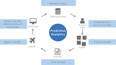
Simply put, predictive analytics is the way that you have to predict any future event based on past behavior. The truth is that predictive analytics is a combination of both statistics and data mining. Therefore, the tools that predictive analytics uses come from these two areas and they include:

predictive-analytics

– build models to predict what can happen in the future

– identify trends and patterns

– create visual representations of the information

– generate other useful information.

Check out the best statistics calculators.

The Goals Of Predictive Analytics

While predictive analytics has many different goals, one of the most important ones is to assign a predictive score (or probability) for the likelihood that a specific organizational unit such as a component, a vehicle or a customer, will behave in a specific way. 

learn-more-about-predictive-analytics

Let’s say, for example, that you are a manufacturer and you are trying to determine the probability of a customer to buy a second product. In this case, you would use predictive analytics. Besides this simple example, there are many areas where predictive analytics plays an important role. These include:

– marketing

– travel

– child protection

– actuarial science

– insurance

– telecommunications

– crime prevention

– insurance

– healthcare

– banking and other financial services.

This is how you should conduct a t test in Excel.

One of the things that you need to understand about predictive analytics is that even though it is defined “in the future”, the reality is that it can also be used to analyze past and present behavior. For example, predictive analytics can be used to analyze the data collected in a crime scene to generate a profile for the most likely suspects. 

Important Areas Where Predictive Analytics Is Used
predictive-analytics-working

While predictive analytics can be used in a wide range of fields, the two most important areas include:

#1: Marketing Analytics:

Marketing analytics allows you to determine how a business or company is really performing. So, it uses metrics such as:

– Marketing attribution: Identifies user actions (called “events” or “touchpoints”) that contribute in some manner to a certain outcome.

– Customer lifetime value (CLTV): Predicts how much a customer will buy over time.

– Quarterly or yearly sales forecasts

– Overall marketing effectiveness

– Next best offer or product recommendation: predicts what your customer is most likely to purchase next

– Return on Investment (ROI).

Learn everything you need to know about an unpaired t tat for two samples.

#2: Healthcare Analytics:

Healthcare analytics includes a wide range of data that is generated by healthcare professionals, patients, and healthcare systems. Healthcare analytics can include keeping and analyzing:

– Financial costs such as supply chain, revenue, costs, and insurance reimbursements

– Data on mass customization of care

– Patient wellness management records

– Biometrics usage

– Patient satisfactory surveys.

Check out this paired t test example.

Predictive Analytics Real Life Examples

what-is-predictive-analytics

One of the best real life examples that w can provide you is related to banking. After all, you just need to think about your credit score. Your past behavior will help determine your present and future behavior in terms of the likelihood of making timely payments in the future. 

Another example is related to cybersecurity, for example. As you know, this is a growing concern and predictive analytics can be used here as well. After all, real-time analytics examines the network traffic and tries to identify patterns that may indicate computer-software vulnerability or fraud. 


The Monte Carlo Simulation

The Monte Carlo simulation, also known as the Monte Carlo Method or the Monte Carlo Sampling, is one of the many ways that you have at your disposal to determine the risk in quantitative analysis and in decision making. 

Monte-Carlo-Simulation

The Monte Carlo simulation is a method that allows you to determine all the possible outcomes of your decisions while, at the same time, it assesses the impacts of the risk. 

Discover the best probability calculators.

The Monte Carlo simulation uses intensive statistical sampling methods. Therefore and due to their complexity, they are, in most cases, only performed with the use of a computer. 

The Monte Carlo simulation is complex because: 

– The input model needs to be simulated hundreds or thousands of times and where each and every simulation needs to be equally likely. 

– The Monte Carlo simulation doesn’t only transform numbers from a random number generator as it also takes these sequences and makes then repeat after a certain number of samples. 

When you use the Monte Carlo simulation, you will be able to determine all the possible events that will or could happen as well as the probability of each possible outcome. 

What is normal distribution?

How Is The Monte Carlo Simulation Use In Real Life

Monte-Carlo-simulation-and-probability

Since the Monte Carlo simulation will deliver you a quantified probability, this means that it also delivers you scenarios with numbers that you can definitely use. 

Let’s say that you are looking to build a factory close to the wetlands and that you want to discover if it will affect the local bird life. In this case, a quantified probability could be something like if you build a new factory, there are about 60% chance that the bird population is affected. As you can see, this is a lot more precise than to simply state that the bird population will be affected. And this is what you get from the Monte Carlo simulation. 

Discover everything you need to know about the Probability Theory. 

Here are the different areas and industries where you can successfully use the Monte Carlo simulation:

– Estimating the transmission of particles through matter

– Assessing risk for credit or insurance

– Analyzing radiative heat transfer problems

odds-vs-probability

– Simulating proteins in biology

– Foreseeing where prices of securities are likely to move

– Calculating the probability of cost overruns in large projects

– Analyzing how a network or electric grid will perform in different scenarios.

Check out this ultimate guide to descriptive analysis.

The Monte Carlo Simulation Accuracy

When you are looking at probabilities, it is important that you use a method that is accurate. And this is exactly the case of The Monte Carlo Simulation. After all, there are many different factors that lead to ensure that The Monte Carlo Simulation is able to hit the exact mark. These include:

– Usually, there are several unknowns in the system

– It usually includes a lot of data

– Since we are determining a probability, there is always a margin of error related to the results that is accepted. 

The truth is that there are times when The Monte Carlo Simulation can drive you into a bad result. This may occur when:

probabilities

– the underlying risk factors aren’t complete 

-you are using an unrealistic probability distribution or when you are using an incorrect model

– the random number generator that you chose for the method isn’t good enough

– using the Monte Carlo simulation isn’t suited to your data

– there are computer bugs.


Everything You Need To Know About Normal Distribution

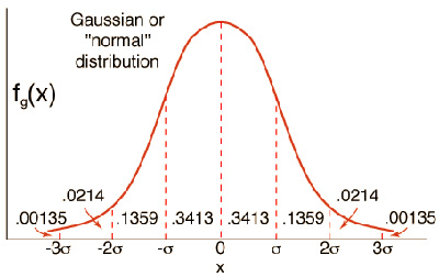
A normal distribution is one of the most used concepts in statistics. So, what exactly is normal distribution?

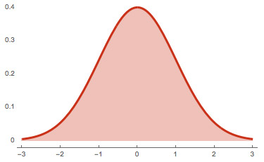
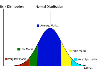
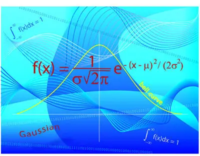
Simply put, a normal distribution is just a distribution that occurs in a natural way in many situations. It is also called the bell curve. 

normal-distribution

Use the best stats calculators for free.

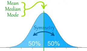
One of the things that you need to keep in mind about the normal distribution is that this curve is symmetrical. This means that half of the data will b on the left of the mean and the other half will be at the right of the mean. 

The normal distribution is very used for many different purposes. In fact, it is commonly used in statistics, business, and even in government bodies such as the FDA. It is often used to compare IQ scores, blood pressure, heights of people, salaries, measurement errors, points on a test, among so many others.  

These are the basic statistics for data science that you need to know.

Properties Of The Normal Distribution

normal-distribution-properties

These are the main normal distribution properties:

– The curve of the normal distribution is symmetric at the center which is around the mean. 

– The median, mode, and mean and all equal.

– The total area under the curve is 1.

– Half of the values ate to the right of the center and the other half of the values are to the left of the center. 

Standard Normal Model

#1: The Distribution Of Data:

One of the best ways that you have to determine if you have a normal distribution or not is to plot the data in a graph. 

When you see that the data is evenly distributed, then you can definitely draw the bell curve or the normal distribution curve. 

Looking for the best Data Science statistic books?

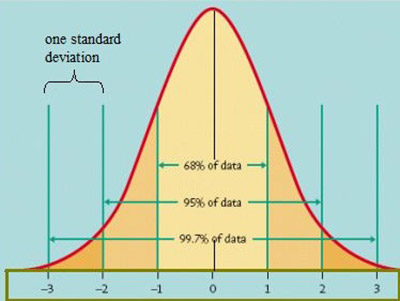
Notice that this curve needs to have a bigger percentage on its inner part and a smaller percentage towards the points on both tails. 

According to the Standard Normal Model, the tails should represent about 5% of your data each while the remaining 90% should be in between. 

#2: Practical Applications:

While it is important that you understand normal distribution as well as how it is drawn and formed, the truth is that an example is always a good way to demonstrate a concept. 

Let’s imagine that you are trying to discover the subjects that you need to work more to improve your grades. One of the most common mistakes people do is that they assume that when you get a score in one subject that is higher than the score you got on a different subject, they are better in the subject where you got a higher score. While this may be true sometimes, this isn’t always the case. 

Learn more about statistical questions.

standard-normal-distribution-standard-deviation

The truth is that all that you can say when this happens is that you are better is a specific subject if you are able to get a score with a certain number of standard deviations above the mean. If you remember, the standard deviation is able to tell you how your data can or cannot be clustered around the mean. 

Let’s say that you just got a score of 90 in Science and 95 in Math. So, you may believe that you need to work harder in Science and that you are better in Math. Nevertheless, you need to know that in Science, your score is 2 standard deviations above the mean. In what concerns to Math, your score is only 1 standard deviation above the mean. 

your-grades

So, with all this information, we can say that your result in Science is far better than your result in Math. After all, your result falls into the tails, being above average. 


What Is The Probability Theory

The Probability Theory is one of the many branches of mathematics that concerns with the analysis of random phenomena. 

Probability-Theory

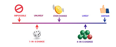
When a random event occurs, you don’t know the outcome. However, you know that there may be several outcomes. So, the Probability Theory helps you determine how likely it is for one of those outcomes to occur. 

The ultimate statistics website you need.

Applying The Probability Theory

One of the things that you need to know and understand about the Probability Theory is that when an experiment can be repeated under similar conditions, it can lead to different outcomes on different trials. 

The group of all the possible outcomes of an experiment is named “sample space”. Let’s say that you want to conduct an experiment tossing a coin. You know that you will have a sample space with two possible outcomes: heads and tails.  

Discover the most common probability math problems.

In case you decide to toss two dice, you know that you will have a sample space with 36 possible outcomes. Each one of these possible outcomes can be named an ordered pair (i, j), where both i and j can assume the values of 1, 2, 3, 4, 5, and 6. 

dices

When we are using the Probability Theory, it is important that both dice are different. They can have different colors, for example. This way, you know that the outcome (3, 1) is different from the outcome (1, 3). However, if you are trying to determine the probability of the event of the sum of the faces showing on the two dice equals six, you will have five different possible outcomes: (1, 5), (2, 4), (3, 3), (4, 2), and (5, 1).

But there are more examples where we can use the Probability Theory. On this one, we will use a drawing of n balls from an urn. This urn includes several balls of different colors. The reality is that this simple example allows providing a good guidance for many different events that may occur in real life. After all, we can use this example as a basis to better understand sample surveys or opinion polls. 

What is a statistical question?

Let’s say that you identify candidate 1 to an election with a ball of a specific color, candidate 2 is identified with a ball of a different color, and so on. So, according to the Probability Theory, you can learn about the electoral preferences of a specific population using simply a sample drawn from that same population. 

balls-in-urns

The Probability Theory, specifically this simple urn draw, is also used with clinical trials. These can be used to determine if a new surgery, a new drug or a new treatment for a disease is better than the standard treatment. 

Take a look at the basic statistic formulas that you need to understand.

tossing-a-coin

However, there are also other experiments that have infinite possible outcomes. Just think about when you want to toss a coin up until tails appear for the first time. This is the kind of experiment that can serve as the basis for measurements such as marginal income, reaction time, temperature, voltage, volume, among others. After all, these ate all made on continuous scales. So, if you keep measuring the different objects or the same object at different times, this can lead to different outcomes. So, we can say that the Probability Theory is also a powerful tool when you need to study this variability. 


The Ultimate Guide To Descriptive Statistics

Simply put, descriptive statistics is a way that you have to summarize and organize the data that you collect. This way, it will be easier to understand it. 

Descriptive-Statistics

A lot of people tend to use descriptive statistics and inferential statistics in the same way. However, the two concepts are different. When you use descriptive statistics, you are looking for a way to describe the data but you aren’t trying to make any kind of inferences from the sample that you are looking at to the whole population. 

The best statistical calculators are available here.

The Different Types Of Descriptive Statistics

Overall, we can easily divide descriptive statistics into two different categories:

#1: Measures Of Central Tendency:

Measures-Of-Central-Tendency

Within this descriptive statistics category, you can assume that there is a number that is central to the set or that is the best representation of the entire set of measurements. 

Learn more about determining the measures of central tendency.

Here are some examples of measures of central tendency:

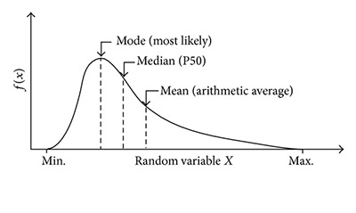
Mean: The mean is simply the number around which the entire data is spread out. In this case, only a number – the mean – can be seen as the best representation of the whole data. 

Median: When you divide your set of data in two equal parts, you get one number at the medium which is called the median. Notice that in order to determine the median, the numbers of the set should be organized in an ascending or descending order. In case the number of terms of the set is odd, the median is the middle term; in case the number of terms of the set is even, the median will be equal to the average of the two middle terms. 

Check out these statistical questions examples.

Mode: Simply mode, the mode is the term that appears more time on the data set. 

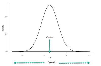
#2: Measures Of Variability (Spread):

Measures-Of-Variability-(Spread)

The measures of variability assume that your data includes some variability. 

Here are some examples of measures of variability or spread: 

Standard Deviation: The standard deviation shows how the data is spread out from the mean So, in order to calculate the standard deviation, you needs to set the difference between each quantity and the mean. When you have the standard deviation is low, this means that the data points are closer to the mean of the data set. On the other hand, when you get a high standard deviation, the data points are spread out over more values and not concentrated around the mean only. 

Understanding what a statistical question is.

Mean Absolute Deviation Or Mean Deviation: This is the average of the absolute differences between each value and the average of all values of your data set. 

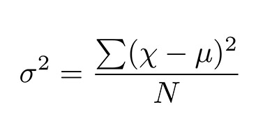
Variance: The variance is simply the square of the standard deviation. So, we can also say that the variance is the square of the average distance between each quantity and mean. 

variance-formula

Range: The range is the difference between the lowest and the highest value of your data set. 

Percentile: When you want to represent the position of the values that you ave on your data set, you can use the percentile. Notice that when you want to calculate the percentile, you need to have your data set in ascending order. 


How To Conduct A T Test In Excel

As you probably already know, a t test can be very useful in statistics. After all, this test allows you to know if there is a difference between the means. In case you don’t know, or simply don’t remember, the bigger the t value, the bigger the difference between the two samples.

Use the best statistic tables. 

While you can do a t test by hand, you should know how to do a t test in excel. After all, this can save you a lot of time. However, you need to understand that when you are working with excel, you can actually make three different t tests:

  • the paired two sample for means
  • the two-sample assuming equal variances
  • the two-sample assuming unequal variances

So, let’s discover how to do a t test in excel.

how-to-do-a-t-test-in-excel

Let’s say that you just collected the data and that you organized the data in your excel spreadsheet. The range A1:A21 contains the first set of values and the B1:B21 contains the second set f values.

Lear more about the two sample t test.

Step #1: Make sure that you choose the “Data Analytics” and then “Data”.

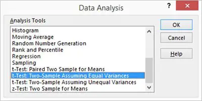
Step #2: Now, you should be able to see the Data Analysis dialog box. So, all you need to do is to pick the t test that you want to make from the Analysis Tools list.

Data-Analysis-dialog-box

As you can see, you’ll be able to choose between:

  • the t-Test: Paired Two-Sample For Means: This is the one that you should choose when you want to make a paired two-sample t test.

  • the t-Test: Two-Sample Assuming Equal Variances: This is the t test that you should choose when you believe that both samples’ means are equal.
  • the t-Test: Two-Sample Assuming Unequal Variances: This is the t test that you need to choose when you want to do a two-sample t test and you believe that the two-sample variances are different.

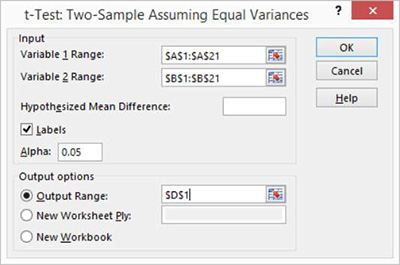
Step #3: As soon as you decide about the test to perform, just click ok. Let’s say that you chose the second t test. You will then see the following dialog:

second-t-test

While this is just an example, the other dialog windows are very similar so you shouldn’t have any problems filling them in.

Discover everything you need to know about the unpaired t test.  

Step #4: Adding The Inputs:

As you can see, the first fields that you need to fill are the “Variable 1 Range” and the “Variable 2 Range”. All you need to do is to fill in with the ranges that you have for the data. In this case, in the first field you will need to add $A$1:$A$21 and in the second field, $B$1:$B$21. However, to make it easier, you can simply drag the data for the appropriate field directly from the excel spreadsheet.

Check out this simple paired t test example.

The next field that you need to fill is the “Hypothesized Mean Difference”. In this box, you will need to specify whether you believe the means are equal or different. The way that you have to do this is very simple. In case you believe that the means are the same, you just need to add zero (0) in the text box. On the other hand, if you believe they are different, you should add the mean difference.


Next, you need to add the Alpha. This refers to the confidence level that you are using in your t test calculation. The confidence level always varies between 0 and 1. So, you will need to add your own. Please notice that if you don’t add any, the default confidence level will be applied – which is equal to 0.05, which is the same to say that you have a 5% confidence level.

The last area that you need to fill regards to the “Output Options”. And these are simply the place where you want your results to be seen. If you want the results to be displayed in a specific cell, you just need to add it right beside the “Output Range”. Or you can choose one of the other options.

Step #5: Click OK.

As soon as you click OK, the results of the t test will be displayed according to what you specified.


Paired T Test Example

The truth is that doing a paired t test is not as difficult as it may seem when you first look at it. Nevertheless, a paired t test example is always a good way to learn exactly what you need to do.

One of the things that you need to have in mind os that a paired t test is used to compare the means of two populations.

Use the top stats calculators.

The paired t test is very used in many different areas. You can use it to compare different health treatments, to analyze the results of a diagnostic test before and after a specific module, among so many others.

paired-t-test-example

Before we actually show you the paired t test example, let’s see how you need to proceed.

Let’s say that you have a sample of n students. They had to do a diagnostic test before module A and another one after completing it. Our goal is to determine the importance of teaching in the student’ skills and knowledge, evaluated with their scores.

Let’s also consider that:

x – represents the diagnostic test score before Module A

y – represents the diagnostic test score after Module A

In order to start testing the null hypothesis, which is the mean difference is zero, here are the steps you need to take:

Step #1: Calculate the difference between the two observations, before and after the diagnostic test, on each pair:

d = y – x

Learn more about the unpaired t test.

Step #2: Determine the mean difference

Step #3: Determine the standard deviation of the differences. Then, you will need to use this value to calculate the standard error of the mean difference:

standard-error-of-the-mean-difference-formula

Step #4: Determine the t-statistic, by using the following formula:

t-statistic-formula

Please remember that you are testing the null hypothesis. Therefore you need to use the t-distribution with n-1 degrees of freedom.

Step #5: Compare your T value with the tn-1 value that you can check on the t-distribution tables.

What is a 2 sample t test? 

Now, let’s check a practical paired t test example:

Let’s say that we are assuming that we want to measure the results of teaching on students as well and that we already know their scores before and after the Module A was taught. Let’s also consider that we are considering a sample of 20 students. So, n = 20.

Here are the scores that the students had:

StudentPre-Module ScorePost-Module ScoreDifference
11822+4
22125+4
31617+1
42224+2
51916-3
62429+5
71720+3
82123+2
92319-4
101820+2
111415+1
121615-1
131618+2
141926+7
1518180
162024+4
171218+6
182225+3
191519+4
201716-1

In the last column, you can already see the calculations of the differences of the scores for each student. So, all you need to do know is to determine the mean difference, using the formula we provided above.

We can then say that the mean difference is 2.05.

So, by using the values and replacing them in the standard deviation of the differences formula also provided above, you will get:

Sd = 2.837

Now, it’s time to determine the standard error of the mean:

SE(d) = Sd / √n = 2.837 / √20 = 0.634

Discover the top intro statistics books. 

Finally, you will need to perform the t-statistic:

t = 2.05 / 1.634 = 3.231

Please notice that this is the t-statistic calculated for 19 degrees of freedom.

So, by looking at the tables, you can see that you will get a p = 0.004.

With this result, we can say that module A does lead to improvement in the students’ knowledge and skills. In fact, there is even a strong evidence of that.


Understand Unpaired T Test For Two Samples

As you probably already know, a t test is very important in statistics and it tends to be used for a wide variety of subjects and topics. Since it can be used as a very broad test, the truth is that there are some derivations of this test, specifically the unpaired t test.

But what exactly is the unpaired t test?

Simply put, the unpaired t test allows you to compare the means of two different samples. However, in order to perform this test, the values need to follow the Gaussian distribution.

unpaired-t-test

Besides, there are some assumptions that you can withdraw when the unpaired t test was performed:

Check out the most important stats calculators that you need. 

#1: The Two Populations Have The Same Variances:

When you perform an unpaired t test, you assume that both populations have different variances as well as the same standard deviation. While this may not mean much for you so far, you will learn that when populations have different variances this fact can be as important as discovering that they have different means.

#2: The Data Needs To Be Unpaired:

Whenever you have data that is a match or paired, you should use the paired t test instead.

Discover the basic statistics that you need to know about for data science.

#3: You Can Only Compare Two Groups:

One of the most common mistakes statistics students make when they are learning more about t tests and the unpaired t test is to use the unpaired t test multiple times in a row. However, this is something that you should avoid or you’ll be increasing the risk of finding a statistically significant difference by chance. Ultimately, this will make it harder for you to interpret both the statistical significance level as well as the P-value. When you need to make multiple comparisons, a better approach is to use the one-way ANOVA.

So, how do you do an unpaired t test?

As you already know, an unpaired t test is used when you want to compare two population means. Usually, this is how you will see the notations:

n1, n2 – refer to the sample sizes of population 1 and 2, respectively

x¯1, x¯2 – refer to the sample means of population 1 and 2, respectively

s1, s2 – refer to the standard deviation of population 1 and 2 respectively.

Here is how the procedure of carrying out an unpaired t test works:

1. You will be assuming that the null hypothesis states that the two population means are equal. Or:

H0: x¯1 = x¯2

2. The first thing that you will need to do is to determine the difference between the two sample means, or:

x¯1 – x¯2

3. Next, you will need to take a closer look at the standard deviation. However, you won’t be looking at the standard deviation of each one of the samples individually. Instead, you will need to calculate the pooled standard deviation:

pooled-standard-deviation-formula

4. In this step, you will need to determine the standard error of the difference between the two means. So, you will need to use the following formula:

standard-error-of-the-difference-between-the-two-means

5. Now, it is finally time to determine the t-statistic. You can easily do it by using the formula:

t = ( x¯1 – x¯2 ) / SE ( x¯1 – x¯2 )

Please note that when you are testing the null hypothesis, you already know that the t will follow a t-distribution with n1 + n2 – 2 degrees of freedom.

Learn more about statistical questions. 

6. Finally, you will need to use the t-distribution tables to compare the value of the t that you got with the tn1+n2−2 distribution. This will give you the p-value for the unpaired t test.

As you ca see, the unpaired t test is easily done. While it includes multiple steps, it is very simple to perform. Nevertheless, if you are seeing all this information for the first time, it may be a bit harder to understand this test without any values. So, let’s take a look at an example of an unpaired t test.

Unpaired T Test – Practical Example:

Let’s say that a company decided to do a study about the number of calories included in the hotdog meat. The truth is that not all hotdog meat is the same and there are some brands that use beef and others that use poultry. So, as you can imagine, the calories contained in both dogs should be different.

After processing the data, the company presented the following data:


GroupSample SizeSample MeanSample Standard Deviation
Beef20156.8522.64
Poultry17122.4725.48

Since we believe these values can follow the Gaussian distribution, we can then proceed with the unpaired t test that we just described above.

1. Let’s start by determining the difference of the means: x¯1 – x¯2

In this case, x¯1 – x¯2 = 156.85 − 122.47 = 34.38

2. Now, it is time to determine the pooled standard deviation. By replacing the numbers of the table into the formula directly:

Sp = √ [[ (n1-1)s1^2 + (n2-1)s2^2 ] / n1 + n2 – 2] = √ [[ (19)22.64^2 + (16)25.48^2 ] / 35] = 23.98

3. Now, in order to determine SE(¯x1 − x¯2):

SE(¯x1 − x¯2) = Sp√ [ (1/n1) + (1/n2) ] = 23.98√[ (1/20)+(1/17) ] = 7.91

What exactly is a statistical question?

4. Finally, you can now calculate the value of the T:

t = ( x¯1 – x¯2 ) / SE ( x¯1 – x¯2 )

t = 34.38/7.91

5. By checking the tables of the t-distribution with 35 degrees of freedom, you will easily discover that p<0.001. So, we can say, almost for sure or with a high degree of certainty, that poultry dogs have fewer calories than beef hotdogs.

Even if you are just learning statistics and the unpaired t test for the first time, we believe that you now have a good knowledge about this specific test and that you won’t have any problems with the procedure.


Two Sample T Test Explained

Before we even start talking about a 2 sample t test, it is important that you understand what a t-test is and what is its purpose in statistics. Simply put, a t test is a hypothesis test that allows you to compare means.

So, based on this simple definition, you can easily understand that a 2 sample t test is another hypothesis test that served to compare means but with the difference that you have two random data samples.

Take a look at the best statistics calculators.


2-sample-t-testOne of the main reasons why researchers and statistics tend to use the 2 sample t test is when they need to evaluate the means of two different groups or variables and understand if these means differ or are the same. For example, the 2 sample t test is very used to determine the effects of receiving a treatment of males versus females.

One of the main advantages of using a 2 sample t test is the fact that you can use it with small and large data samples.

Now that you already understand what a 2 sample t test is and what its purpose is, it is time to see it in action. The reality is that there are two common applications for the 2 sample t test:

Learn more about quantitative reasoning questions and answers.

#1: Using The 2 Sample T Test To Determine That The Means Are Equal:

When you are looking to use this test to see if the means of the two samples of data you collected are the same, you need to follow the next steps:

Step 1. Define The Hypothesis:

The following table shows three different of hypothesis: three nulls and three alternatives.

SetNull HypothesisAlternative HypothesisNumber of Tails
1μ1 – μ2 = dμ1 – μ2 ≠ d2
2μ1 – μ2 > dμ1 – μ2 < d1
3μ1 – μ2 < dμ1 – μ2 > d1

As you can see, each one of this hypothesis shows the difference (d) between the mean of the two populations – μ1, the mean of population 1, and μ2 the mean of the population 2.

Step 2. Determine The Significance Level:

While you can use any value between 0 and 1, most researchers tend to use0.10, 0.05 or 0.01 as the significance level.

Step 3. Determining The Degrees Of Freedom (DF):

While you may see that the degrees of freedom can be determined in a simpler way, in order to be more exact, you should use the following formula:

DF = (s1^2/n1 + s2^2/n2)^2 / { [ (s1^2 / n1)^2 / (n1 – 1) ] + [ (s2^2 / n2)^2 / (n2 – 1) ] }

When you are determining the degrees of freedom using this formula, you may not get an integer. In this case, you need to make sure that you round it off to the nearest whole number.

Looking for the best introductory statistics books?

Step 4. The Test Statistic:

In order to compute the test statistic, you will need to use the following formula:

test-statistic

test-statistic-2

d – refers to the hypothesized difference between the means of the population

s1 – refers to the standard deviation of sample 1

s2 – refers to the standard deviation of sample 2

n1 – refers to the size of sample 1

n2 – refers to the size of sample 2

Step 5. Determine The P Value:

In case you don’t know, the P-value is just the probability of observing a specific sample statistic as extreme as the test statistic.

Step 6. Evaluating The Results:

The result of the test will come from the comparison between the P-value with the significance level. So, in case the P-value is less than the significance level, the null hypothesis is rejected.

#2: Using The 2 Sample T Test To Determine The Difference Between Means:

In this case, you need to make sure that you comply with the following rules so that you know that you can perform a 2 sample t test:

  • the samples are independent
  • the sampling method that was used for each sample was the simple random sampling
  • the population distribution is normal
  • the population needs to be at least 20 times larger when compared with its sample
  • the sampling distribution seems to be approximately normal.

If all these conditions are met, you can start the 2 sample t test by following the next steps:

Step 1. State The Hypothesis:

On the following table, you can see three different sets of data where you have both the null and alternate hypothesis. Please notice that this is a similar table to the one we showed before.

SetNull HypothesisAlternative HypothesisNumber of Tails
1μ1 – μ2 = dμ1 – μ2 ≠ d2
2μ1 – μ2 > dμ1 – μ2 < d1
3μ1 – μ2 < dμ1 – μ2 > d1

In this case, you can see that the set 1 and the sets 2 and 3 are different. This is why we will need to to use a two-tailed test for the set 1 and the next 2 sets need to be tested using a one-tailed test.

When we want to have the null hypothesis to say that the means of the different populations are the same, which is the same as saying that d=0, then you can have the null and alternate hypothesis like this:

Ho: μ1 = μ2

Ha: μ1 ≠ μ2

Step 2. Defining The Analysis Plan:

In order to have your analysis plan all set, you need to ensure that you considered several elements:

  • The Significance Level, which, again, you should use 0.10, 0.05 or 0.01.
  • The Test Method, which you will need to use the 2 sample t test.

Learn how to calculate the P value from Z. 

Step 3. Analysis Of Sample Data:

The analysis of sample data includes discovering the standard error, the degrees of freedom, determining the test statistic, and finally determining the P-value that is associated with the test statistic. Here’s how it is done:

  • Standard Error: Just use the following formula:

standard-error

where,

s1 – is the standard deviation of sample 1

s2 – is the standard deviation of sample 2

n1 – is the size of sample 1

n2 – is the size of sample 2

  • Degrees Of Freedom: You just need to use the formula above.
  • Test Statistic: Just use the following equation of the t statistic (t):

test-statistic

test-statistic-2

  • P-Value.

Step 4. Interpreting The Results:

In order to interpret the results, you will need to compare the P-value with the significance level. In case the P-value is inferior, which is what happens most of the times, you will reject the null hypothesis.

The last concept that you need to know about when we are talking about a 2 sample t test is the paired t test formula concept. Simply put, while you will use the 2 sample t test when you have two completely different populations, you will have to use the paired t test when the samples that you have are connected in some way.


Discovering Z Test Example Problems

One of the first concepts that you will learn when you are studying statistics is the Z test. But can you tell some Z test example problems?

Before we answer this question, it is important to remember what the Z test is and what it should be used for.

Looking for a statistical calculator?

Simply put, the Z test is a statistical procedure that allows you to test the different or alternate hypothesis against the null hypothesis. While the null hypothesis is the one that the researcher tries to reject and usually reflects the common view of the subject, the alternate hypothesis is what the researcher thinks is the cause of a certain phenomenon.

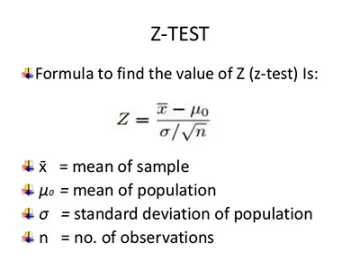
In order to solve any Z test example problems, you need to make use of the Z test formula:

z-test-example-problems

One of the things that is always important to have in mind when you are considering doing a Z test is that you need to have a large sample. The truth is that since we are trying to prove the validity of the null hypothesis, you need to make sure that you have a good population size to have a complete view of the problem that you are trying to solve. The larger the sample of the population you get, the lower are the odds of getting a wrong conclusion.

Ultimately, you will use a Z test when:

  • the samples are randomly drawn
  • you know the standard deviation
  • the number of observations is large
  • the samples are taken from a population, independently.

Z Test Example Problems

Let’s say that a teacher is convinced that his students have an IQ above average. So, he randomly picked 30 students and they have a mean score of 112.5. Is this enough to prove that the teacher is right?

Please notice that the mean population IQ is 100 and that the standard deviation is 15.

#1: Stating the different hypothesis:

– The Null Hypothesis: We accept the fact that the mean population IQ is 100. So,

H0: μ = 100

– The Alternate Hypothesis: We want to see of the students have an above average IQ. So,

H1: μ > 100

This is how you determine the standard deviation. 

#2: Draw A Chart:

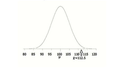
One of the things that can really help you solve a Z test problem is by drawing a picture to visualize your data:

z-test-chart-visualization

#3: The Alpha-Level:

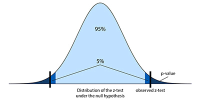
In this case, no one said anything about the alpha-level. So, when this happens, you need to assume that the alpha-level is 0.05.

So, in this case, you would have a Z-score = 1.645

Learn how to find the Z score for a normally distributed data. 

#4: Using The Z-test Formula:

z-test-example-problems

Z = (112.5 – 100) / (15 / √30 ) = 4.56

#5: Conclusions:

z-test-example-problems

Since 4.56 is greater than 1.645, you will reject the null hypothesis, making the teacher’s claim right.

These are the basic statistic formulas that you need to know. 

As you can see, making a Z test doesn’t need to b complicated at all. We understand that we showed you a simple example and that real-life problems can get a bit trickier. However, with experience and by understanding the Z-test basics, you will easily be able to solve any related problems.