Category : Blog

How To Deal With Missing Data In Statistics

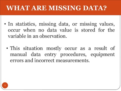
When you are learning statistics and studying simple models, you are probably not aware that missing data is something very common in statistics. The reality is that date from experiments, surveys, and other sources are often missing some data. 

missing-data-1

One of the most important things to keep in mind about missing data in statistics is that the impact of this missing data on the results depends on the mechanism that caused the data to be missing. 

Looking for the best statistics calculators?

Data Are Missing For Many Reasons

  • Subjects in longitudinal studies tend to drop out even before the study is complete. The reason is that they may have either died, moved to another area, or they simply don’t see a reason to participate. 
  • In what concerns surveys, these usually suffer from missing data when participants skip a question, don’t know, or don’t want to answer. 
  • In the case of experimental studies, missing data occurs when a researcher is unable to collect an observation. The researcher may become sick, the equipment may fail, bad weather conditions may prevent observation in field experiments, among others. 

Discover how to interpret the F test.

Why Missing Data Is Important In Statistics
Why-Missing-Data-Is-Important-In-Statistics

Missing data is a very important problem in statistics since most statistical procedures require a value for each variable. Ultimately, when a data set is incomplete, the data analyst needs to decide how to deal with it.

In most cases, researchers usually tend to use complete case analysis (also called listwise deletion). This means that they will be analyzing only the cases with complete data. Individuals with data missing on any variables are dropped from the analysis.

While this is a simple and easy to use approach, it has limitations. The most important limitation, in our opinion, is the fact that it can substantially lower the sample size, leading to a severe lack of power. This is especially true if there are many variables involved in the analysis, each with data missing for a few cases. Besides, it can also lead to biased results, depending on why the data are missing.

Learn why adding values on a scale can lead to measurement error.

Missing Data Mechanisms
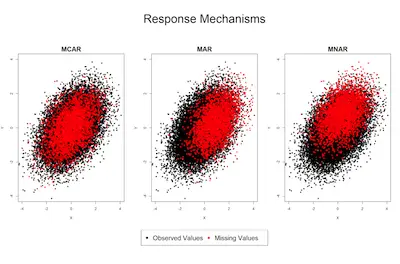
Missing-Data-Mechanisms

As we already mentioned above, the effects on your model will depend on the missing data mechanism that you decide to use. 

Overall speaking, these mechanisms can be divided into 4 classes that are based on the relationship between the missing data mechanism and the missing and observed values. 

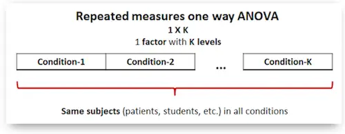
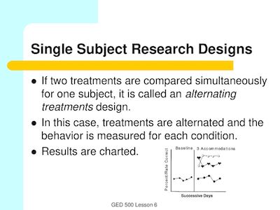
These 3 designs look like repeated measures.

#1: Missing Completely At Random (MCAR): 

MCAR means that the missing data mechanism is unrelated to the values of any variables, whether missing or observed.

Data that are missing because a researcher dropped the test tubes or survey participants accidentally skipped questions are likely to be MCAR. Unfortunately, most missing data are not MCAR.

#2: Non-Ignorable (NI):

NI means that the missing data mechanism is related to the missing values.

It commonly occurs when people do not want to reveal something very personal or unpopular about themselves. For example, if individuals with higher incomes are less likely to reveal them on a survey than are individuals with lower incomes, the missing data mechanism for income is non-ignorable. Whether income is missing or observed is related to its value.

#3: Missing At Random (MAR):

MAR requires that the cause of the missing data is unrelated to the missing values but may be related to the observed values of other variables.

MAR means that the missing values are related to observed values on other variables. As an example of CD missing data, missing income data may be unrelated to the actual income values but are related to education. Perhaps people with more education are less likely to reveal their income than those with less education.
How To Interpret Regression Coefficients

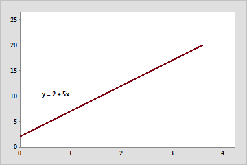
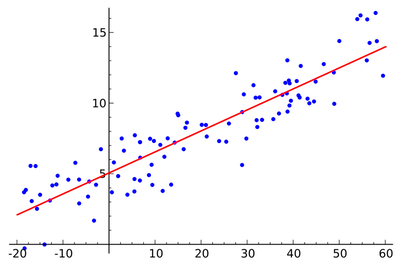
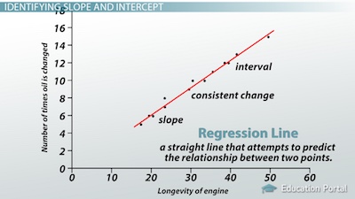
When you are learning statistics, you are probably already familiar with linear regression. After all, it is one of the most popular statistical techniques. However, while it seems pretty simple and obvious, the reality is that interpreting regression coefficients of some models may be difficult. 

Discover all the statistics calculators you can use.

How To Interpret Regression Coefficients

regression-coefficients

To help you overcome these difficulties in interpreting regression coefficients, let’s try to interpret the coefficients of a continuous and a categorical variable. 

Notice that while we are using the linear regression, you can apply the same basics to interpret the coefficients from any other regression model without interactions. 

Learn more about the binomial distribution.

Linear Regression

Linear-Regression

As you probably already know, a linear regression model with two predictor variables can be expressed with the following equation:

Y = B0 + B1*X1 + B2*X2 + e

The variables in the model are:

  • Y, the response variable;
  • X1, the first predictor variable;
  • X2, the second predictor variable; and
  • e, the residual error, which is an unmeasured variable.

The parameters in the model are:

  • B0, the Y-intercept;
  • B1, the first regression coefficient; and
  • B2, the second regression coefficient.

One simple example would be a model of the height of a shrub (Y) based on the amount of bacteria in the soil (X1) and whether the plant is located in partial or full sun (X2).

Let’s consider that the height is measured in cm, bacteria is measured in thousand per ml of soil, and the type of sun = 0 if the plant is in partial sun and type of sun = 1 if the plant is in full sun.

Imagine that the regression equation was estimated as follows:

Y = 42 + 2.3*X1 + 11*X2

Discover the differences between descriptive and inferential statistics.

Interpreting The Intercept

Interpreting-The-Intercept

B0, the Y-intercept, can be interpreted as the value you would predict for Y if both X1 = 0 and X2 = 0.

This means that we would expect an average height of 42 cm for shrubs in partial sun with no bacteria in the soil. But it is important to notice that this is only a meaningful interpretation in case both X1 and X2 can be 0. Besides, the data set also needs to include values for X1 and X2 that were near 0.

In our example, it is easy to see that X2 sometimes is 0, but if X1, our bacteria level, never comes close to 0, then our intercept has no real interpretation.

Looking to know more about confidence intervals?

Interpretation Of Coefficients Of Continuous Predictor Variables

Since X1 is a continuous variable, B1 represents the difference in the predicted value of Y for each one-unit difference in X1, if X2 remains constant. So, as you can easily understand, if X1 differed by one unit (and X2 did not differ) Y will differ by B1 units, on average.

Looking back at our example, shrubs with a 5000 bacteria count would, on average, be 2.3 cm taller than those with a 4000/ml bacteria count, which likewise would be about 2.3 cm taller than those with 3000/ml bacteria, as long as they were in the same type of sun.

Interpretation Of Coefficients Of Categorical Predictor Variables

Now, if we take a look at B2, it can be interpreted as the difference in the predicted value in Y for each one-unit difference in X2 if X1 remains constant. However, since X2 is a categorical variable coded as 0 or 1, a one unit difference represents switching from one category to the other. We can then state that B2 is the average difference in Y between the category for which X2 = 0 (the reference group) and the category for which X2 = 1 (the comparison group).

So compared to shrubs that were in partial sun, we would expect shrubs in full sun to be 11 cm taller, on average, at the same level of soil bacteria.


Understanding The Binomial Distribution

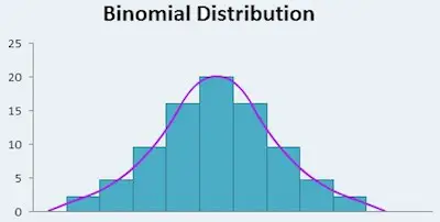
Simply put, the binomial distribution is a probability distribution that shows you the likelihood that a value will take one of two independent values under a given set of parameters or assumptions. 

Take a look at the best statistics calculators online. 

binomial-distribution

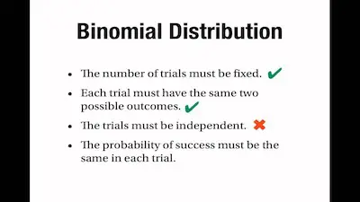
When talking about the binomial distribution, it is important to keep in mind that it has some underlying assumptions:

  • there is only one outcome for each trial
  • each trial has the same probability of success
  • each trial is mutually exclusive or independent of each other.

In addition, the binomial distribution is the opposite of a continuous distribution such as the normal distribution. After all, it is a common discrete distribution. 

Looking Into The Binomial Distribution

Looking-Into-The-Binomial-Distribution

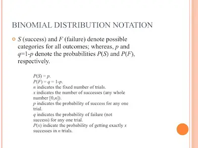
Notice that when you are using the binomial distribution, you need to know that it only counts two different states. generally speaking, these are usually represented by 1 when there is success and by 0 when there is failure. 

So, we can then say that the binomial distribution represents the probability for x successes in n trials, given a success probability p for each trial. 

When you are using the binomial distribution, you will be summarizing the number of trials or observations when each trial has the same probability of attaining one particular value. The binomial distribution will then determine the probability of observing a specified number of successful outcomes in a specified number of trials.

Understanding the difference between the Z score and the T score.

When To Use The Binomial Distribution

When-To-Use-The-Binomial-Distribution

While you can use the binomial distribution in many different situations, it tends to be mainly used in social science statistics as a building block for models for dichotomous outcome variables. Some examples include if someone will die within a specified period of time or even if Democrats or Republicans will win the upcoming election. 

Where to get the best statistics help online? 

Analyzing The Binomial Distribution

Analyzing-The-Binomial-Distribution-1

When you want to calculate the expected value of a binomial distribution (or mean), you need to know that you will need to multiply the number of trials by the probability of successes. 

Let’s say that the expected value of the number of heads in 50 trials of head and tales is 25 (50 X 0.5). 

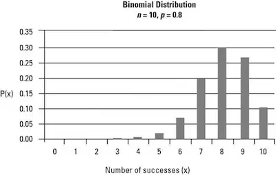
The mean of the binomial distribution is np, and the variance of the binomial distribution is np (1 − p). This means that:

  • When p = 0.5, the distribution is symmetric around the mean. 
  • When p > 0.5, the distribution is skewed to the left. 
  • When p < 0.5, the distribution is skewed to the right.

Learn how to use descriptive analysis in research.

In addition to this, the binomial distribution is the sum of a series of multiple independent and identically distributed Bernoulli trials. In a Bernoulli trial, the experiment is said to be random and can only have two possible outcomes: success or failure. Flipping a coin is therefore considered to be a Bernoulli trial; each trial can only take one of two values (heads or tails), each success has the same probability (the probability of flipping a head is 0.5), and the results of one trial do not influence the results of another. The Bernoulli distribution is a special case of the binomial distribution where the number of trials n = 1.


Descriptive Vs. Inferential Statistics

One of the first things that you study when you begin learning statistics is the descriptive vs inferential statistics difference. 

Discover the statistics calculators you need.

descriptive-vs-inferential-statistics

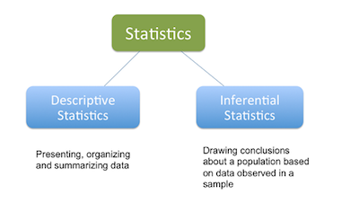
The reality is that when you are analyzing data such as the marks achieved by 100 students for a piece of coursework, it is possible to use both descriptive and inferential statistics in your analysis of their marks. But what is descriptive statistics, inferential statistics, and the differences and similarities between the two?

Descriptive Statistics

Descriptive-Statistics

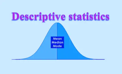
Simply put, descriptive statistics is the analysis of data that helps describe, summarize, or show data in a meaningful way. This way, you can see patterns emerging from the data itself. However, unlike what you may thing, descriptive statistics doesn’t allow you to draw any conclusions beyond the data that you analyzed or reach conclusions regarding any hypotheses you might have made. 

Notice that this doesn’t make descriptive statistics less important. In fact, descriptive statistics is important because if you simply presented your raw data, it would be hard to visualize what the data was showing, especially if there was a lot of it. 

Learn more about confidence intervals.

For example, if you had the results of 100 pieces of students’ coursework, you may be interested in the overall performance of those students. You would also be interested in the distribution or spread of the marks. And this is exactly what descriptive statistics shows you. 

Typically, there are two general types of statistic that are used to describe data:

  • Measures of central tendency: these are ways of describing the central position of a frequency distribution for a group of data. You can describe this central position using a number of statistics, including the mode, median, and mean. 
  • Measures of spread: these are ways of summarizing a group of data by describing how spread out the scores are. To describe this spread, a number of statistics are available to us, including the range, quartiles, absolute deviation, variance and standard deviation.

Discover how to interpret the F-test.

Inferential Statistics

Inferential-Statistics

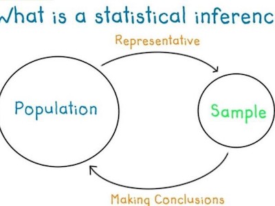
As we just saw above, descriptive analysis allows you to look at a group or part of a population’s data. You can then use different statistics to reach some conclusions. However, in the real world, it is almost impossible to access the whole population data that you are interested in investigating. Therefore, you are limited to a group which means that you will need to use a sample of the population that can represent that same population. 

We can then say that inferential statistics are techniques that allow you to use these samples to make generalizations about the populations from which the samples were drawn. The process of achieving this is called sampling. Inferential statistics arise out of the fact that sampling naturally incurs sampling error and thus a sample is not expected to perfectly represent the population. The methods of inferential statistics are the estimation of parameter(s) and testing of statistical hypotheses.


Looking to know why adding values on a scale can lead to measurement error?

Descriptive Vs. Inferential Statistics – Bottom Line

Descriptive-Vs.-Inferential-Statistics-Bottom-Line

Overall speaking, it is understandable that descriptive statistics are limited. This means that you can only make conclusions about the population that you actually measured. 

In the case of inferential statistics, we need to mention that they have 2 limitations. The first one which is also the most important one is the fact that you are providing data about a population that you have not fully measured, and therefore, cannot ever be completely sure that the values/statistics you calculate are correct. The second limitation is the fact that inferential statistics requires the researcher to make educated guesses to run the tests. 


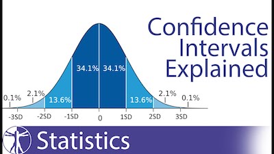
Understanding Confidence Intervals

One of the most important statistics concepts is confidence intervals. But what is a confidence interval after all?

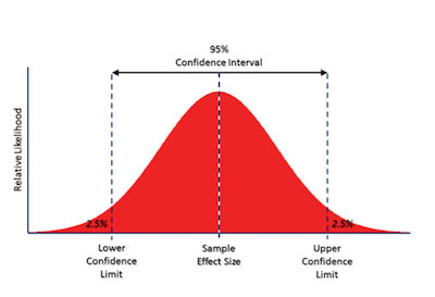
Simply put, a confidence interval refers to the probability that a population parameter will fall between two set values for a certain proportion of times. So, we can then say that confidence intervals measure the degree of uncertainty or certainty in a sampling method. 

confidence-intervals

It’s always important to keep in mind that a confidence interval can take any number of probabilities, with the most common being a 95% or 99% confidence level.

Discover the best statistics calculators online.

Why We Need Confidence Intervals 

When you are learning a new concept for the first time, you often question yourself about what’s the point in learning it. Well, in the case of confidence intervals, statisticians look at them to measure uncertainty. 

Why-We-Need-Confidence-Intervals

Here’s a simple example: a researcher chooses different samples randomly from the same population and computes a confidence interval for each sample. As you can easily understand, the resulting datasets are all different. The reality is that some intervals include the true population parameter and others do not.

Check out our confidence interval calculation for population mean. 

So, in sum, a confidence interval is simply a range of values that likely would contain an unknown population parameter. So, ultimately, a confidence interval refers to the percentage of probability, or certainty, that the confidence interval would contain the true population parameter when you draw a random sample many times. 

Should confidence intervals or tests of significance be used?

Calculating A Confidence Interval

calculating-a-confidence-interval

Let’s say that some researchers are studying the heights of high school softball players. The first thing they will do is to take a random sample from the population (the team of softball players) and let’s imagine that they establish a mean height of 74 inches. 

The mean of 74 inches is a point estimate of the population mean. The truth is that you can’t actually use this point estimate by itself because it does not reveal the uncertainty associated with the estimate. So, you are missing the degree of uncertainty in this single sample.

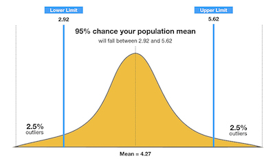
The reality is that confidence intervals deliver more information than point estimates. After all, by establishing a 95% confidence interval using the sample’s mean and standard deviation, and assuming a normal distribution as represented by the bell curve, the researchers arrive at an upper and lower bound that contains the true mean 95% of the time. 

Discover how to find a confidence interval.

Let’s say that the interval is between 72 inches and 76 inches. If the researchers take 100 random samples from the population of high school softball players as a whole, the mean should fall between 72 and 76 inches in 95 of those samples.

Besides, in the case that the researchers want even greater confidence, they can expand the interval to 99% confidence. Doing so will create a broader range, as it makes room for a greater number of sample means. 

So, if they establish the 99% confidence interval as being between 70 inches and 78 inches, they can expect 99 of 100 samples evaluated to contain a mean value between these numbers. A 90% confidence level means that we would expect 90% of the interval estimates to include the population parameter. Likewise, a 99% confidence level means that 95% of the intervals would include the parameter.


How To Interpret The F-Test Of Overall Significance In Regression Analysis

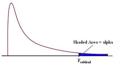
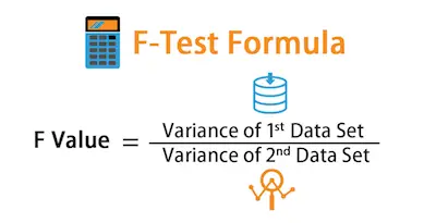
Simply put, the F-test of overall significance tells you whether your linear regression model is a better fit to the data than a model that contains no independent variables. So, today, we decided to take a step further and tale a look at how the F-test of overall significance fits in with other regression statistics, such as R-squared. 

Find all the statistics calculators you need here.

F-test

In case you don’t know or simply don’t remember, the R-squared tells you how well your model fits the data, and the F-test is related to it.

Understanding The F-Test

One of the things that statistics students need to keep in mind is that the F-test is a statistical test that is incredibly flexible. This means that you can actually use it in a wide range of settings. One of the main advantages of using the F-test is that it allows you to compare the fits of different linear models which is something that t-tests don’t do.

Check out our F-value calculator.

Calculating The F-Test Of Overall Significance

When you need to calculate the F-test of overall significance, you just need to use your statistical software and add the right terms in the 2 models that it compares. 

F-Test-Formula

Notice that the overall F-test compares the model that you specify to the model with no independent variables. This type of model is also known as an intercept-only model.

When you need to run the F-test for overall significance, it will have two hypotheses:

  • The null hypothesis states that the model with no independent variables fits the data as well as your model.
  • The alternative hypothesis says that your model fits the data better than the intercept-only model.

In statistical output, you can find the overall F-test in the ANOVA table. 


Understanding a bit more about the F test.

Interpreting The Overall F-Test Of Significance

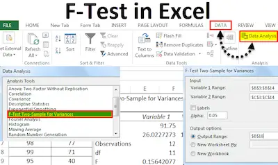
F-Test-in-Excel

In order to interpret the results of the test, you will need to compare the p-value for the F-test to your significance level. In case the p-value is inferior to the significance level, this means that your sample data delivers enough evidence to conclude that your regression model fits the data better than the model with no independent variables. In case you are wondering, this is good news. After all, it means that the independent variables in your model improve the fit.

Overall speaking, when none of your independent variables are statistically significant, this means that the overall F-test is also not statistically significant. 

In some situations, tests may produce conflicting results. This can occur because the F-test of overall significance assesses all of the coefficients jointly whereas the t-test for each coefficient examines them individually. These conflicting test results can be hard to understand. 

Here’s an F-test example.

Additional Way To Interpret The F-Test Of Overall Significance

It is also important to keep in mind that when you have a statistically significant overall F-test, you can also draw other conclusions. 

When you have a model with no independent variables, for example, you can easily conclude that all of the model’s predictions equal the mean of the dependent variable. Therefore, if the overall F-test is statistically significant, your model’s predictions are an improvement over using the mean.


Why Adding Values On A Scale Can Lead To Measurement Error

When some statistics students look at a multi-item scale to measure a construct, they are lead in error and they, sometimes, start adding values on a scale. But this shouldn’t be done at all. Instead, a key step is to actually create a score for each subject in the data set. 

Discover the best online statistics calculators you need.

Simply put, this score is an estimate of the value of the latent constructor or factor the scale is measuring for each subject. In case you haven’t seen it yet, we are actually running the final step of a Confirmatory Factor Analysis.

adding-values-on-a-scale

When you are looking for the simplest way to create a score, you will need to either average or add up the values of each variable on the indicator or scale for each subject. This is called a factor-based score. It’s based on the factor in the factor analysis, but is not technically a factor score since it doesn’t use the factor weights. But the problem is that this method is far away from being able to be accepted. 

Why Adding Values On A Scale Can Lead To Measurement Error

The best estimate of the subject’s value on the latent construct you’re measuring with your observed indicator variables is the true factor score. After all, the factor loadings, as calculated by the analysis, determines the optimal weighting for each indicator.

Make sure to use out standard error calculator.

Notice that when the EFA/CFA and structural equation models “predict” the factor scores it uses a linear regression, incorporating the factor loadings into the model.

So, here’s an example when you need to compare the difference between the “add up the scores” and linear regression approach. We will use five indicators together model the latent construct of Assertiveness:

AS3   Automatically take charge

AS4   Know how to convince others

AS5   Am the first to act

AS6   Take control of things

AS7   Wait for others to lead the way

The table below gives the coefficients generated by the linear regression approach. For the addition method, the mean of the linear regression coefficients was used to evenly weight the variables.

table

The two approaches will not generate similar scores. If you check it closely, the AS3’s weighting is 52% greater and AS4 is – 47% less using linear regression compared to addition.

Discover how to calculate standard error. 

Notice that if the factor loadings are all equal, it makes sense to use addition. In this particular case, we can add up the scores for each indicator to generate the factor scores. However, we cannot assume they are equal without testing them.

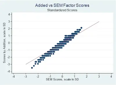
While we believe we have explained this concept well, we also believe that taking a look at it visually may help you understand the concept better. So, in this visual, we will be comparing the factor scores generated by a structural equation model and adding the indicator scores together. 

The factor scores generated by the structural equation model are standardized, with a mean of zero and a standard deviation of 1. To compare the addition approach scores we will standardize them as well.

Looking for the standard error calculation online?

scatterplot-of-the-SEM-and-addition-generated-scores-1

As you can see, we have a scatterplot of the SEM and addition generated scores. Notice that the diagonal line represents the line where the scores generated by the two methods are equal.

If you take a closer look at the image above, you can see that there are very few points on the diagonal line and the generated scores aren’t the same. 


3 Designs That Look Like Repeated Measures

When you first hear or read about the repeated measures concept, most statistics students tend to immediately assume that it can be applied to a wide range of situations. However, the truth is that it describes only one situation. 

Simply put, a repeated measures design is one where each subject is measured repeatedly over time, space, or condition on the dependent variable. To add to this fact, it is important to keep in mind that these repeated measurements aren’t independent of each other. In fact, they are clustered. Besides, they are more correlated to each other than they are to responses from other subjects. Even if both subjects are in the same condition. 

repeated-measures

Discover all the stat calculators you need.

So, when you want to get accurate standard errors, p-values, and confidence intervals, then the non-independent clustering needs to be accounted. While this may seem simple, the truth is that it can easily become complicated since the clustering can look very different in different studies. In addition, it is also worth pointing out that some study works look like repeated measures but they’re not. 

Repeated Measures – What They Need To Comply With

Ultimately, you have repeated measures only if you have 3 different and important elements:

  1. Multiple clustered measurements of the dependent variable
  2. that are more correlated to each other than to others’ measurements because they’re measured on the same subject
  3. repeatedly over time, space, or condition.

So, when you have a study and you want to determine if it requires a repeated measures analysis, then you need to define these 3 elements. Let’s check some examples:


Make sure to use our standard error calculator.

Example #1: Measuring the graduation rate in 50 high schools in the 4 years before and 4 years after an intervention:

  1. Multiple clustered measurements of the DV: 8 measures of pass rate per school
  2. Subject: school
  3. Repeated over: time


Discover our standard error calculator updated in 2020.

Example #2: Measuring the time it takes second language learners to read a sentence under 4 different grammar structures:

  1. Multiple correlated measurements of the DV: 4 measures of reading time of each sentence per person
  2. Subject: Person learning a language who reads the sentences
  3. Repeated over: grammar structure condition

Studies That Aren’t Repeated Measures

#1: A Single Subject That Is Measured Over Time:

A-Single-Subject-That-Is-Measured-Over-Time

One of the cases where many statistics students tend to assume they can use the repeated measures is when they have a single subject that is measured over time. However, this design is missing the second element. The truth is that the responses from our single subject cannot be more correlated to each other than to other subjects’ responses because there are no other subjects.

Simply put, this is a time series which means that there is a serial autocorrelation (similarities in responses that are closer in time). 


Discover how to calculate standard error. 

#2: A New Random Sample Of Subjects At Each Time Point:

A-New-Random-Sample-Of-Subjects-At-Each-Time-Point

Another case that many students tend to assume the use of repeated measures is a cross-sectional longitudinal design. For example, you measure the annual revenue of 30 companies for 10 years. But each year you randomly selected a new sample of 30 companies. That’s not repeated measures. With new subjects at each time point, we’re missing element #2.

When you cannot match a subject’s measurement in year 1 to the same subject’s measurement in year 2, that is not repeated measures. 

#3: A Predictor Variable Is Measured Repeatedly Over Time For each Subject But The Dependent Variable Is Measured Once:

For example, a study where 30 companies’ revenues over 10 years were used to predict whether or not they had an IPO in year 11.

In this case, it is missing element #1. The repeated measurements have to be on the dependent variable. Since you have only a single measurement of the dependent variable, that’s not repeated measures, even though there are 10 measures of the predictor.


Z Score Vs T Score: Understanding The Difference

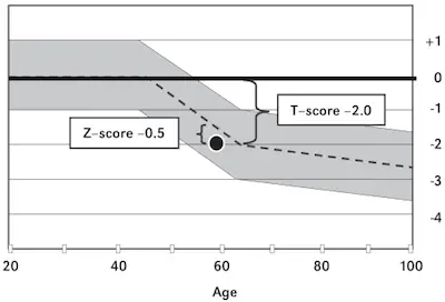
When you are learning statistics, there are two different but important concepts that you will learn: the z score and t score. However, according to the emails and messages that we get, we have a clear idea that many students find it difficult to understand the differences between z score vs t score. So, today, we decided to tell you a bit more about both the z score and the t score as well as what is the main difference between them. In addition, and in what concerns to the more practical aspect of statistics, we will also show you when you should use the z score and when you need to use the t score. 

z-score-vs-t-score

Use all the best stats calculators in just one place.

So, if you have some difficulties to understand the z score vs t score differences or even some difficulties in understanding these main concepts, make sure to keep reading. 

Z Score Vs T Score

Simply put, both the z score and the t score are both used in hypothesis testing. And this is probably the reason why so many statistics students struggle to know which one to use. 

Generally speaking, in elementary stats, you tend to use more the z score in testing than the t score. Nevertheless, it is important to understand both. 

Discover everything you need to know about the z score table.

What Is A Z Score?

What-Is-A-Z-Score

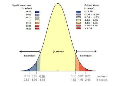
The z score, which is also known as the standard score, gives you an idea about how far from the mean a data point is. In case you want to be more technical, then you can say that the z score is a measure of how many standard deviations below or above the population mean a raw score is. 

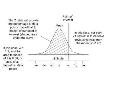
One of the most important aspects to keep in mind about the z score is that it can be placed on a normal distribution curve. As you probably already know, z scores range between -3 standard deviations that would be when they fall to the far left of the normal distribution curve and up to +3 standard deviations, which is when they fall to the far right of the normal distribution curve. 

When you need to use a z score, you need to know the mean μ as well as the population standard deviation σ.

Learn how to use the standard normal distribution table.

Notice that z scores are a popular way to compare results to a normal population. As you know, results from tests or surveys have thousands of possible results and these may often seem meaningless. While you may know that you weigh 100 pounds, this is simply meaningless unless you compare it with the average population’s mean weight. 

What Is A T Score?

What-Is-A-T-Score

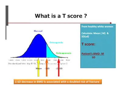
The t score or t statistic is used in a t test when you are trying to either support or reject the null hypothesis. If you think about it, you can actually see some similarities with the z score. After all, you need to find a cut off point, find your t score, and then compare the two. You use the t statistic when you have a small sample size, or if you don’t know the population standard deviation.

One of the main ideas to keep in mind about the t score is that it doesn’t tell you much on its own; it needs to be put in some context. So, with this in mind, you need to actually get more information by taking a sample and running a hypothesis test. 

Check out everything you need to understand and use the standard normal table.

Z Score Vs T Score: Understanding The Difference

Z-Score-Vs-T-Score-Understanding-The-Difference

So, now that we showed you a simplified version of what the z score and the t score are, you are probably wondering about when you should use one or the other. 

As a rule of thumb, you should use the t score whenever you have a sample size below 30, and when you have an unknown population standard deviation. On the other hand, whenever you have a sample size that is 30 or more and you know the standard deviation of the population, then you need to use the z score. 


Examples Of Z Score Calculations

When you are studying statistics, z score calculations are an important part. The truth is that the z score calculations are useful for many different things and you need to ensure that you understand the concepts well. 

Discover the best statistics calculators.

One of the most basic things that you will learn in statistics is how to find the z score for some value of a normally distributed variable. So, today, we decided to show you some examples of z score calculations so you can better understand the concept. But before we begin with the examples, it is always useful to give you a brief insight into z scores. 

Why We Use The Z Score

z-score-calculations

One of the most pertaining questions that many statistics students have is why do we need to learn and understand z scores. 

Notice that while there is only one standard normal distribution, there is an infinite number of normal distributions. Therefore, the main goal of calculating the z score is to relate a specific normal distribution to the standard normal distribution. 

As you probably already know, the standard normal distribution has been being studied for a very long time and there are tables that provide areas underneath the curve – the z score tables. These are the ones that you need to use when you are doing your z score calculations.

Check out the standard normal table.

Since there is an universal use of the standard normal distribution, it is incredibly important to standardize a normal variable. So, you can see the z score as the number of standard deviations that are away from the mean of your distribution. 

The Z Score Formula

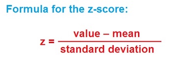
The formula that we use to calculate the z score is: 

z = (x – μ)/ σ

Where:

  • x is the value of our variable
  • μ is the value of our population mean.
  • σ is the value of the population standard deviation.
  • z is the z-score.


Take a look at a z score table.

Examples Of Z Score Calculations

looking-at-the-z-tables

Now that we already took a look at the z score concept, it is time to do some z score calculations. This is the best thing you can do to ensure that you understand the concept of the z score. 

Let’s say that you know about a population of a particular breed of cats having weights that are normally distributed. Furthermore, suppose that you also know that the mean of the distribution is 10 pounds and the standard deviation is 2 pounds. 

In the first example, you want to know the z score for 13 pounds. How can you know this?

Simply put, you will simply need to replace the x = 13 into your z-score formula. With that said:

z = (13 – 10)/2 = 1.5

This means that 13 is one and a half standard deviations above the mean.

Check out the standard normal distribution table.

What about if you want to know the z score of 6 pounds? 

As you can easily understand, the process is pretty similar to the previous one. All you need to do now is to replace the variable by 6 instead of 13. 

The result is:

z = (6 – 10)/2 = -2

We can then state that 6 is two standard deviations below the mean.

standard-normal-distribution

What about if you now want to know how many pounds corresponds to a z score of 1.25?

While this may seem a bit trickier question, the reality is that you now know the z score. So, in this case, you will need to solve the formula for x:

1.25 = (x – 10)/2

Multiply both sides by 2:

2.5 = (x – 10)

Add 10 to both sides:

12.5 = x

So, you can see that 12.5 pounds correspond to a z-score of 1.25.