Category : Blog

Sampling Variability – What Is It And Why It Is Important

In life, you can’t always get what you want, but if you try sometimes, you get what you need. In what concerns to statistics, this is also true. After all, while you may want to know everything about a population or group, in most cases, you will need to deal with approximations of a smaller group. In the end, you need to hope that the answer you get is not that far from the truth. 
sampling-variability

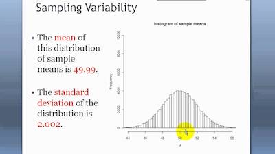
The difference between the truth of the population and the sample is called the sampling variability.

When you are looking for a quick and simple definition for sampling variability, then you can state that it is the extent to which the measures of a sample differ from the measure of the population. However, there are certain details that you need to keep in mind. 

Looking At The Parameters And Statistics

When you are looking at measures that involve a population, you need to know that it is incredibly rare to measure them. For example, you just can’t assume that you can measure the mean height of all Americans. Instead, what you need to do is to take a random selection of Americans and then actually measure their mean height. 
Looking-At-The-Parameters-And-Statistics

Check out our online p-value calculator for a student t test.

Knowing this mean height means that you already have a parameter. So, you can then say that a parameter is just the value that refers to the population like the mean, deviation, among others, that you just don’t know. 

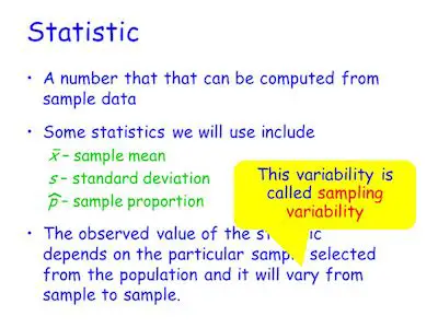
Notice that it is impossible to measure a parameter; what you do have is a possible estimate using statistics. This is why a measure that refers to a sample is called a statistic. A simple example is the average height of a random sample of Americans. As you can easily understand, the parameter of the population never changes because there is only one population. But a statistic changes from sample to sample. 

Looking for a t-statistic and degrees of freedom calculator?

What is Sampling Variability?

If you recall, sampling variability is the main purpose of this blog post. However, we needed to take a look at the previous concepts (statistics and parameters) to ensure that you understand what sampling variability is. 

Simply put, the sampling variability is the difference between the sample statistics and the parameter. 

Whenever you are looking at a measure, you can always assume that there is variability. After all, variability comes from the fact that not every participant in the sample is the same. For example, the average height of American males is 5’10” but I am 6’2″. I vary from the sample mean, so this introduces some variability.

Generally, we refer to the variability as standard deviation or variance.

The Uses Of Sampling Variability
The-Uses-Of-Sampling-Variability

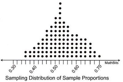
As you can imagine, you can use sampling variability for many different purposes and it can be incredibly helpful in most statistical tests. After all, the sampling variability gives you a sense of different the data are. While you may not be in the average height since you may be taller, the truth is that there are also people who are shorter than the average height. And with sampling variability, you can know the amount of difference between the measured values and the statistic. 

Here’s the best standard deviation calculator.

In case the variability is low, it means that the differences between the measured values and statistics are small, such as the mean. On the other hand, if the variability is high, it means that there are large differences between the measured values and the statistics. 

As you probably already figured out, you are always looking for data that has low variability. 

Sampling variability is used often to determine the structure of data for analysis. For example, principal component analysis analyzes the differences between the sampling variability of specific measures to determine if there is a connection between variables.

Time Series Analysis and Forecasting Definition and Examples

While many students tend to struggle in statistics, we believe that the topics aren’t that hard to learn and understand. All it takes is to keep a few concepts in mind and then take a look at different examples so you can see them in practice. 

Learn more abou statistics here.

time-series-analysis-and-forecasting

Two of the areas that we believe cause a lot of problems to statistics students are time series analysis and forecasting. However, as you are about to discover, these concepts are simple and easy to understand. Hopefully, at the end of this post, you won’t have any more problems with them. 

What Is Time Series?

What-Is-Time-Series

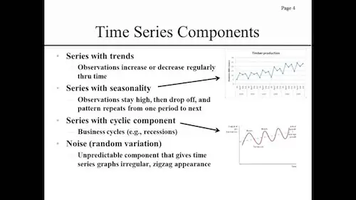
Simply put, a time series is just a set of data recorded at regular times. Let’s say that you decided to record the outdoor temperature at noon every single day for 1 year. The movement of the data over time may be due to many independent factors:

What is heteroscedasticity?

#1: Cyclical Movements: 

These cycles can take many years to play out. They include the known business cycles and while some may only take 6 others, others can take half a century. 

#2: Long Term Trend:

This is when you are looking at the data as a whole, eliminating the noise or the short-term variations. 

#3: Seasonal Variation: 

These are predictable patterns of both ups and downs that occur within a single year but they also repeat year after year. Just think of temperatures for example. ou know that in the Spring and Summer they tend to go up as well as they tend to go down in Fall and Winter. 

Learn hoe to perform a heteroskedasticity test.

#4: Noise: 

All data that you collect has noise. These are the so called random variations or fluctuations due to factors that you cannot control. 

Now that you already understand these factors, you need to put them together. The truth is that each factor has an associated data series: 

  • Trend factor: Tt
  • Cyclic factor: Ct
  • Seasonal factor: St
  • Noise factor: Nt

Finally, the original data series, Yt, consists of the product of the individual factors:

Yt = Tt × Ct × St × Nt

What Is Forecasting?

What-Is-Forecasting

Simply put, when you read forecasting you immediately think of predicting future values of data based on what happened before. 

Notice that this is not a perfect science since there are many factors you can control and that may affect the future values substantially. So, the further into the future you want to forecast, the less certain you can be of your prediction. 


Understanding the significance level.

If you don’t believe us, just watch the weather reporting and you’ll get a hang of it. 

Basically, the theory behind a forecast is as follows:

  1. Smooth out all of the cyclical, seasonal, and noise components so that only the overall trend remains.
  2. Find an appropriate regression model for the trend. Simple linear regression often does the trick nicely.
  3. Estimate the cyclical and seasonal variations of the original data.
  4. Factor the cyclical and seasonal variations back into the regression model.
  5. Obtain estimates of error (confidence intervals). The larger the noise factor, the less certain the forecasted data will be.

Hypothesis Testing for Newbies

When you are conducting statistical analysis, you just can’t go through it without hypothesis testing. 

Learn everything you need about statistics here.

hypothesis-testing

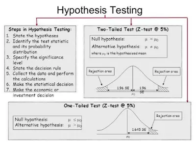
Simply put, hypothesis testing refers to the process where you generate a clear and testable question, collect and analyze appropriate data, and finally draw an inference that answers your question. So, as you can see, there are many different steps you need to go through. 

What Is A Hypothesis?

Overall speaking, a hypothesis is just a possible explanation you may have for patterns that you observe in people or nature. Let’s sat that you spent some time watching people drink coffee and you believe that most people drink more coffee in the morning than in the afternoon. So, when you watch this and you make this statement, you are stating that there is a difference between drinking coffee in the morning and afternoon.

Check out our student t value calculator.

On most occasions, you usually generate a hypothesis from previous research. Besides, it is important to keep in mind that a good hypothesis will propose a relationship between 2 or more variables. 
looking-at-the-hypothesis

Let’s get back to the previous coffee example. 

What you are proposing here is that the time of the day actually affects the amount of coffee people drink. So, in this particular case, time of day is one variable and the number of coffees drank is another variable. Since you believe that the time of the day is the reason for people to drink more or less coffee, then you can assume that the time of day is the independent variable and the amount of coffee is the dependent variable. 

Looking for a z-score calculator?

As soon as you have a clear hypothesis, you can then data so you can look at the pattern you predict. In this case, you would need to collect data on people both in the mornings and afternoons as well as how much coffee they drink at both times. 

accept-or-reject-the-hypothesis

Now that you already collected your data, it is time to analyze it for patterns. In case you see the pattern that you predicted with your hypothesis, then you’re hypothesis was correct. However, you need to be able to state why. On the other hand, if your data doesn’t show the pattern you predicted, then you state that and revise your hypothesis to reflect the pattern in the data.

Easily determine the critical f-value using our simple calculator.

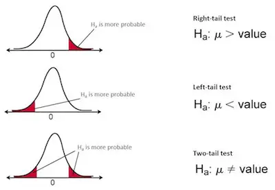
When you are doing hypothesis testing, one of the trickiest parts is determining whether the pattern or model that you find is not only different but different enough to mean something. And this is where the null hypothesis comes in. 

Simply put, a null hypothesis (µ0) is a hypothesis that predicts no difference or pattern between the variables. In our example, the null hypothesis would be that there is no pattern between people drinking coffee and the time of day. If our hypothesis is not right, then the null hypothesis is right, and vice versa.
To determine if the statistical model that you come up with is different enough, we compare it to another sample or the population. In the case of the tired coffee drinkers, we would compare the average number of coffee drinks in the morning to the average number of coffee drinks in the afternoon.


What is Logistic Regression?

When you are conducting a study, there’s nothing better than having all your data nice and straight. After all, you know that when this happens, it is easier to predict outcomes. However, this doesn’t always happen. 

Discover the best online statistics calculators.

logistic-regression

The reality is that sometimes, you want to know how likely something happens and not the actual outcome. So, you need to look at logistic regression.

What is Logistic Regression?

As you probably remember, variables can be either categorical or continuous. Categorical variables are the ones that exist as some sort of discrete unit like multiple choice answers. On the other hand, continuous variables are the ones that exist on some scale like gas mileage or height. 

As you can easily understand, each type of variable has a particular type of statistics linked with them due to their nature. 

Understanding the difference between correlation and linear regression.

In the case of linear regression, you deal with continuous variables. This way, you can analyze the data and predict an outcome based on a scale. However, in what concerns to categorical variables, there are no traditional scales or lines. So, this means you can’t use linear regression. 

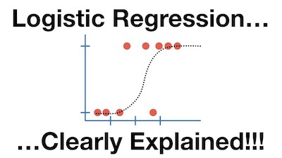
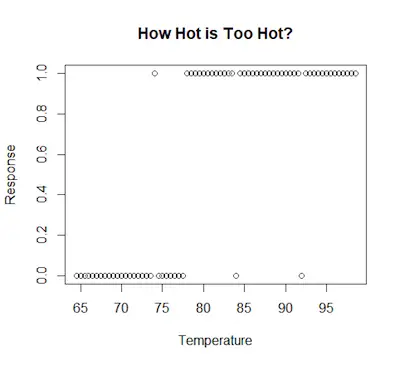
So, when this happens, the first thing you need to look at is binary logistic regression. Let’s take a look at a more practical example. Imagine that you just asked some people if they think the temperature (in Fahrenheit) is too hot. Their answers are expressed in the chart below:

temperature-in-Fahrenheit-graph

As you can see, the data isn’t a normal scatter plot. You can see that the data points aren’t all over the place – they are focused on either 1 or 0 because these were the answers people have to choose from. 

Discover how to perform a simple regression analysis.

This means you can’t calculate the typical line as you would for linear regression because there is no “sort of” response.

Instead, you need to calculate the probability of a person responding either 1 or 0. That is what binary logistic regression is for. We use it to calculate the chance of a person responding to one of two choices.

The general model for binary logistic regression is:

general-model-for-binary-logistic-regression

Where:

  • P(Y) means that we are calculating the probability of an outcome of 1 occurring. 
  • e shows the use of logarithmic functions that create a line of best fit for the data.

So, after running the analysis, your model looks like this:

after-running-the-analysis

Is Your Model Any Good?

One of the things that you always need to keep in mind about logistic regression is that this type of model can’t be interpreted as a linear regression model using R2. 

The truth is that with the logistic regression, you are interested in the probability of an outcome and not in the actual outcome. Therefore, you need to consider the likelihood of an outcome. This is called log-likelihood.

Learn how to interpret regression coefficients.

Simply put, the log-likelihood refers to adding the probability of the predicted outcome to the probability of the actual outcome so that you can get a sense of how well our model explains all the probability of the event occurring.


How To Perform A Heteroskedasticity Test

If statistics were perfect (as you sometimes see on your statistics books), all your data would always follow a nice straight line and you would never have any errors. However, as you already know, in the real world, things just don’t go that way. The truth is that data can be all over the place and follow a rhyme or reason we didn’t predict. This is the reason why you need to look for patterns in the data using test-statistics and regressions. 

heteroskedasticity-test

You can find the best statistics calculators at StatCalculators.

As you can easily understand, to use those statistics, you usually need to meet the assumption that your data is homoskedastic. This means that the variance of the error term is consistent across all measures of the model. Besides, it also means that the data is not heteroskedastic. 

How To Perform A Heteroskedasticity Test

There are a couple of ways to test for heteroskedasticity. So, let’s check a couple of them:

#1: Visual Test:

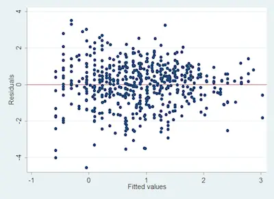
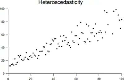
The easiest way to do a heteroskedasticity test is to simply get a good look at your data. Ideally, you generally want your data to follow a pattern of a line, but sometimes it doesn’t. So, the quickest way to identify heteroskedastic data is to see the shape that the plotted data take. 

Don’t know how to perform a simple regression analysis?

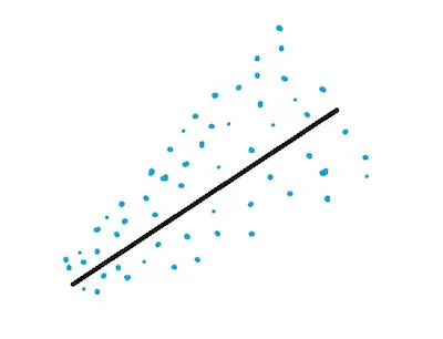
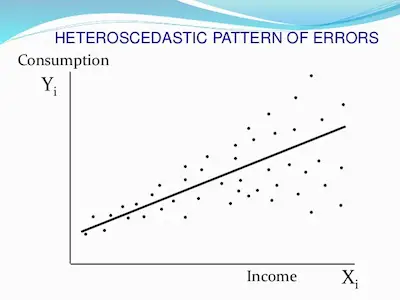
Just check the image below that follows a general heteroskedastic pattern because it is cone-shaped:

general-heteroskedastic-pattern

Since the variance varies, you shouldn’t perform a normal type of linear regression.

#2: Breusch-Pagan Test:

Breusch-Pagan-Test-1

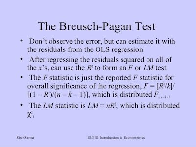
The Breusch-Pagan test is another way you have to do a heteroskedasticity test. The truth is that math is very straightforward:

χ2 = n · R2 · k

Where,

  • n is the sample size
  • R2 is the coefficient of determination based on a possible linear regression
  • k represents the number of independent variables. 
The degrees of freedom are based on the number of independent variables instead of the sample size. This test is interpreted as a normal chi-squared test. 

When you get a significant result, this means that the data is heteroskedastic. Notice, however, that if the data is not normally distributed, then the Breusch-Pagan test may give you a false result. 

Learn how to deal with missing data in statistics.

#3: White’s Test:

White-Test

There’s no question that the White’s test is the most robust test when you are performing a heteroskedasticity test. The reality is that it tests whether all the variances are equal across your data if it is not normally distributed. Notice that the math may be a bit complicated but you can certainly use a statistic software to calculate it for you. 

The White’s test is interpreted the same way as a chi-square test. If the test is significant, then the data is heteroskedastic. Besides, it still determines whether the variance is all equal across the data. However, the test is very general and can sometimes give false negatives.

Learn how to interpret regression coefficients.

Bottom Line

One of the most important things to keep in mind is that determining the heteroskedasticity of your data is essential for determining if you can run typical regression models on your data. Besides, there are 3 main tests you can perform to determine the heteroscedasticity.


What Is Heteroscedasticity?

Heteroscedasticity, which can also be spelled heteroskedasticity, is crucial when you are trying to interpret many things including linear regression. So, today, we decided to take a closer look at heteroscedasticity and see what it is and how you can use it. 

heteroscedasticity

Discover everything you need to know about statistics.

What Is Heteroscedasticity?

Simply put, heteroscedasticity is just the extent to which the variance of residuals depends on the predictor variable. 

If you remember, the variance refers to the difference between the actual outcome and the outcome that was predicted by your model. Besides, in case you don’t know or simply don’t remember, residuals can be different from the model as well. 

We can then say that the data is heteroskedastic when the amount that the residuals vary from the model changes as the predictor variable changes. 

The truth is that many statistics students deal with some difficulties when looking at these definitions and concepts as they are. So, there is nothing like checking an example so you can fully understand what heteroscedasticity is. 

Finally understand the significance level.

Heteroscedasticity – An Example

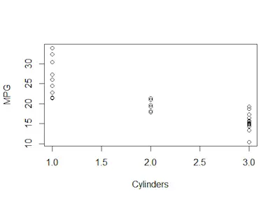
Imagine that you are shopping for a car. One of the most important things people want to know before they buy a new car is the gas mileage. So, with this mind, you decide to make a comparison between the number of engine cylinders to the gas mileage. And you end up with the following graph:

Heteroscedasticity-Graph

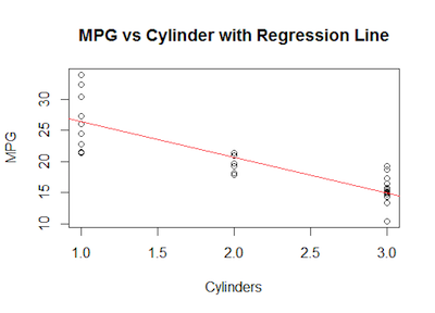
As you can see, there is a general downward pattern. However, at the same time, you can also see that the data points seem to be a bit scattered. It is possible to fit a line of best fit to the data. But there it misses a lot of the data.

Gas-Milleage

If you pay attention to the image above, you can see that the data points are pretty spread out at first. But when you look at the data closer, you see that it spreads out again. This represents heteroscedastic data. So, this means that your linear model doesn’t fit the data very well, so you need to probably adjust it. 

Discover the OLS assumptions.

Why Do You Need To Care With Heteroscedasticity?

The main reason why heteroscedasticity is important is that it represents data that is influenced by something that you are not accounting for. So, as you can understand, this means that you may need to revise your model since there is something else going on. 

Overall speaking, you can check for heteroscedasticity when you compare the data points to the x-axis. When you see that it spreads out, this shows you that the variability of the residuals (and therefore the model) depends on the value of the independent variable. But this is not good for your model. After all, it also violates one of the assumptions of linear regression.

So, whenever this occurs, you need to rethink your model. 

Looking to know more about factorial design basics for statistics?

Special Notes

One of the things that many people don’t know is the fact that if the data can be heteroscedastic, it may also be homoscedastic as well. 

Simply put, homoscedastic data is when the variability of the residuals don’t vary as the independent variable does. So, if your data are homoscedastic, that is a good thing. It means that your model accounts for the variables pretty well so you should keep it.

One common misconception about hetero- and homo-scedasticity is that it has to do with the variables themselves. But it only has to do with the residuals. 


Understanding The Significance Level

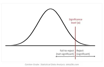
When talking and learning about statistics, you probably already know that significance is paramount to come up with a viable model that explains patterns in your data. So, we can then say that the significance level is the level at which we are willing to accept the chance as an explanation. 

Check out the best statistics calculators online.

significance-level

Before we proceed to talk a bit more about the significance level, we want to ensure that we are on the same page. So, summing up, when you are doing statistical analysis, you need to develop a hypothesis about patterns in your data. You will then use those methods to determine a model of the data that fits the hypothesis. According to what you already know, the null hypothesis is that the model does not fit the data very well while the hypothesis is the model itself. 

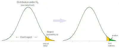
So, when you reject the null hypothesis, this means that you are accepting the hypothesis as true with a specific degree of confidence. That degree of confidence represents the significance level of the model. 

Learn more about the binomial distribution.

What Does Significance Mean?

What-Does-Significance-Mean

Generally, in statistics, we are willing to accept that level of chance. After all, it is very low that I chanced upon the right order. This also means that I am 95% sure that I did not simply guess correctly and I can taste the difference.

So, put another way, the significance level is the amount to which we are willing to attribute our results to chance.

This is the difference between descriptive and inferential statistics.

Why Significance Levels Are Almost Always 5%? Can’t They Be 0%?

Why Significance Levels Are Almost Always 5%? Can't They Be 0%?

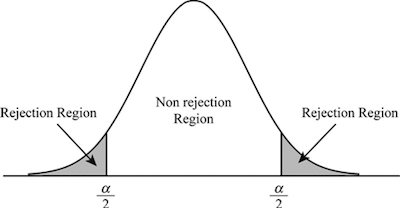
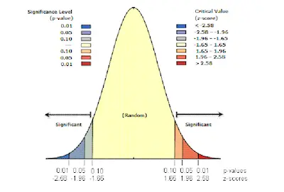
The significance level that most statisticians are willing to accept is 5% or a probability of 0.05. Sometimes, they select a significance level of 0.01 or 0.001. The lower level of chance you accept, the more likely you are to reject the null hypothesis correctly.

But why not just select 0% chance?

In this case, this would mean that there was no error at all, and this is just not feasible over hundreds or thousands of trials. There is always an infinitesimally small chance always present in any experiment or study due to error.

significance-level-visual-interpretation-1

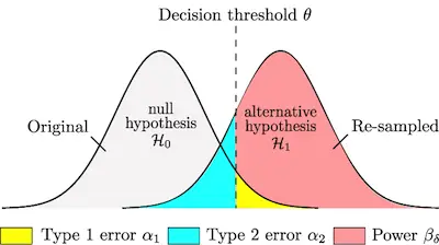
Also, the smaller degree of chance that we are willing to accept increases the chance that we reject or retain the null hypothesis falsely. This is called Type I Error. To compensate, researchers usually accept a small amount of chance at the 5%, 1%, or 0.1% levels.


Learn how to interpret regression coefficients.

Conclusion

As you can see, it’s not difficult to understand the significance level concept. After all, and mathematically speaking, the significance level refers to the probability of getting that event or model by change. Conceptually, the significance level is the degree of confidence that we have in retaining or rejecting our hypothesis of the difference between the model and random chance. 5% is usually the highest significance level that statisticians and researchers are willing to accept, though it can be less. 


OLS (Ordinary Least Squares) Assumptions

One of the first things that you learn about statistics is that there are numerous ways to analyze data. However, as you can easily understand, the way you do it depends not only on what you want to know but also on the data that you actually have. 

Discover everything you need to know about statistics.

OLS-Ordinary-Least-Squares-assumptions

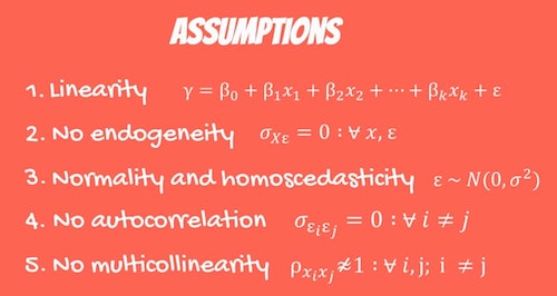
The reality is that one of the most common wats to analyze data is by using regression models. These types of models estimate patterns in the data using something called ordinary least squares (OLS) regressions. As you probably already know, the OLS (Ordinary Least Squares) needs to meet specific assumptions to be valid. 

OLS (Ordinary Least Squares) Assumptions

#1: The Linear Regression Model is Linear In Parameters:

Notice that the expression linear in parameters is a bit tricky. The truth is that it only means that the data follow a linear pattern. So, this is a condition of the correlation of the data. Notice that the data doesn’t need to form an exact line. It simply needs to follow either a positive or negative flow for the most part. 

Learn more about factorial design basics for statistics.

#2: There Is A Random Sampling Of Observations:

There-Is-A-Random-Sampling-Of-Observations

Another important OLS (Ordinary Least Squares) assumptions is the fact that when you want to run a regression, you need to make sure that the sample is drawn randomly from the population. When this doesn’t occur, you are basically running the risk of introducing an unknown factor into your analysis and the model won’t take it into account. 

Notice that this assumption also makes it clear that your independent variable causes the dependent variable (in theory). So, simply put, the OLS is a causal statistical method that investigates the ability of the independent variable to predict the dependent variable. This means that you are looking for a causal relationship instead of a correlation.

Discover how to perform a simple regression analysis.

#3: The Conditional Mean Should Be Zero:

This assumption simply means that the average of your error terms for each measurement needs to be zero. This shows that there is no relationship between the independent variable and the errors. 

#4: There Is No Multi-Collinearity Or Perfect Collinearity:

There-Is-No-Multi-Collinearity-Or-Perfect-Collinearity-1

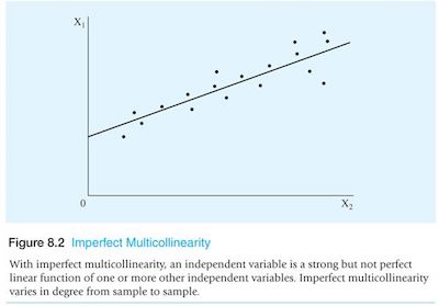
Collinearity means that two or more of your independent variables have a strong correlation with one another. So, when this happens, there is a strong relationship or effect between the two or more variables that you didn’t account for. In this case, your OLS regression can give you a false model. 

How to deal with missing data in statistics?

#5: There Is Homoskedasticity And No Autocorrelation: 

There-Is-Homoskedasticity-And-No-Autocorrelation

In case you don’t know, heteroskedasticity is a measure of the spherical nature of the data. You can actually see it visually if your data shows the shape of a cone instead of a line. 

When your data is heteroskedastic, this means that the variance varies as the data changes. So, since the OLS is based on the variance, you need to ensure that you always have a consistent squared variance and not a changing variance. 

#6: The Error Terms Should Be Normally Distributed:

In case your textbook doesn’t refer to this assumption, it is because it is already covered on the number #3. Nevertheless, we believe that it is important to reinforce it. After all, this means that your errors that are positive cancel out your errors that are negative. This is something that you should check once you have your model.


Factorial Design Basics For Statistics

When you are doing experiments with both physical and social sciences, one of the standards is that you use a random controlled experiment with just one dependent variable. However, there is a limitation to this design: it overlooks the effects that multiple variables can have with each other. 

When this occurs, you can use one of the most popular factorial design basics for statistics – the factorial design analysis of variance which is also known as the factorial ANOVA. 

Discover the best online statistics calculators.

A Simple Example

Let’s say that you just finished a college class in statistics and the final exam has gotten everyone talking about which majors do best – science or arts. At this moment, the class is mixed between art and science majors and underclassmen and upperclassmen. So, you decide to analyze the means of the final exam scores to figure out who is the best.

Learn more about confidence intervals.

The Main Idea Behind Factorial Design Basics For Statistics

If you remember the simple example we mentioned above, you have 2 variables that have an effect over the outcome: major and college experience, and each has two levels in it. So, this means that there are two independent variables and one dependent variable (final exam scores). 

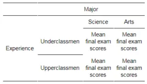
Factorial design was born to handle this kind of design. Besides, the factorial ANOVA compares groups that may interact with one another. Instead of comparing two groups (majors and experience), you are actually comparing 4 groups:

factorial design basics for statistics

Here you have an example of 2 x 2 factorial design ANOVA. This means that there are two factors that we consider independent variables with two levels of treatment each. So, there will be four groups based on the combination of these factors.

Just like ANOVA, you will compare the means using the variances of each group and group level. However, you cannot simply do a series of ANOVAs because that would introduce too much error to confidently say there is a significant difference. So, you should only look for the main effects of each independent variable and how they potentially interact.

Discover how to interpret the F-test of overall significance in regression analysis.

Main Effects And Interactions

One of the best things about factorial analysis is the fact that it allows us to distinguish between main effects and potential interactions in the groups.

In one-way ANOVA, the main effect is present when the groups within a factor demonstrate a significant difference from the grand mean. In our example, the main effect would be a significant difference between upper and underclassmen or a difference between the arts and the sciences. 

An interaction is present when the dependent variable of the group is affected by a combination of both factors. In our example, a possible interaction would be between underclassmen status and being a science major. This would mean that there is a significant difference between this group and the others. 

Learn why adding values on a scale may lead to measurement error.

Looking At The Visual Differences

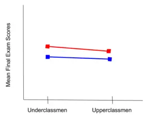
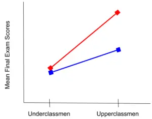
Getting back to our example, we will have two lines: the red one which represents the arts majors, and the blue one which represents the science majors.

first visual difference

In the example above, you can see that the lines are close and almost parallel. This means that there is most likely no significant difference between majors, between college experience, and no interaction.

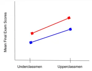
second visual difference

This example indicates that there is a main effect. We know this because, even though the lines are still approximately parallel, the mean final exam scores represent a difference. There is no interaction in this diagram.

third visual difference

Now we have an example of an interaction. The lines are no longer parallel, so there is something going on between the two factors. This is an example of both a main effect and an interaction. You know there is a main effect because the mean final exam scores are different between under and upperclassmen. Since the lines cross (or would if we extend them) there is an interaction between major and college experience.


How To Perform A Simple Regression Analysis

When you have data, most of the time, you should start to analyze it using a graph or some sort of linear regression. However, as soon as you realize, you get an equation. And this is exactly where simple regression analysis comes in. 

simple regression analysis

Discover the best online statistics calculators.

Looking Into The Simple Regression Analysis

Before we take a deeper look at the simple regression analysis, we believe that we should start by reviewing what makes a regression. 

The truth is that simple regression analysis simply refers to the interpretation and use of the regression equation. In case you don’t remember, this is how it looks like:

Learn how to deal with missing data in statistics.

regression equation

The Yi represents the dependent variable in your equation. This refers to the effect or outcome that we are interested in. Xi represents the independent variable and this is the variable that we think predicts the outcome.

In what concerns to the other things, this is where things become more interesting. The b1 represents the actual relationship between the independent and dependent variable. Now, the b0 is more of a theoretical term instead of a practical one. It technically means that when the independent variable is equal to zero, then the dependent variable is equal to b0. 

The last part of the equation is εi. This is the error term or the range of wrongness associated with your equation. However, the error term is usually combined with b0 to make the equation a little easier to use.

Learn more about the binomial distribution.

Simple Regression Analysis

simple regression analysis graph

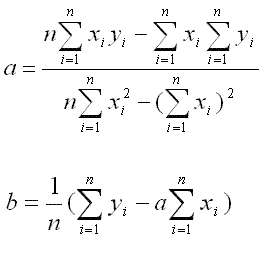
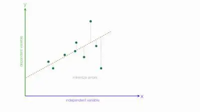
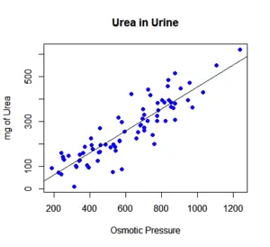
If you take a look at the above graph, you can see a line surrounded by a lot of dots. Each dot represents a data point with an independent variable and a dependent variable. So, using the equation

Linear regression equation

You can come up with just a line that ends up representing the data. 

One of the things that you need to keep in mind is that this line isn’t a perfect fit for the data. Nevertheless, it is still a good prediction. And this is exactly what the regression analysis does: it predicts a dependent based on the independent variable. 

Understand the difference between descriptive and inferential statistics.

How Good Is The Prediction?

When you are calculating the regression equation for the data set that you have, you need to ensure that you also calculate the correlation coefficient. 

Simply put, the correlation coefficient is a value between -1 and +1 which represents the strength of the regression equation’s ability to predict an outcome. 

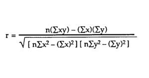
The closer the correlation coefficient is to 1 (either negative or positive), the stronger the relationship, with 1 being a perfect prediction. The formula is:

correlation coefficient formula

Notice that the correlation coefficient is different from the coefficient of determination, r2. Simply put, the coefficient of determination is more explanatory since it tells you how much of the variability in the outcome is due to the variability in the predictor.

Overall speaking, a high coefficient of determination means that most of the variance of the model is explained by the independent and dependent variables. On the other hand, a low coefficient of determination means that there is a lot of variance that the model doesn’t explain.